Hopper is the Transportation Optimization algorithm within Cosmic Frog. It designs optimal multi-stop routes to deliver/pickup a given set of shipments to/from customer locations at the lowest cost. Fleet sizing and balancing weekly demand can be achieved with Hopper too. Example business questions Hopper can answer are:
Hopper’s transportation optimization capabilities can be used in combination with network design to test out what a new network design means in terms of the last-mile delivery configuration. For example, questions that can be looked at are:
With ever increasing transportation costs, getting the last-mile delivery part of your supply chain right can make a big impact on the overall supply chain costs!
It is recommended to watch this short Getting Started with Hopper video before diving into the details of this documentation. The video gives a nice, concise overview of the basic inputs, process, and outputs of a Hopper model.
In this documentation we will first cover some general Cosmic Frog functionality that is used extensively in Hopper, next we go through how to build a Hopper model which discusses required and optional inputs, how to run a Hopper model is explained, Hopper outputs in tables, on maps and analytics are covered as well, and finally references to a few additional Hopper resources are listed. Note that the use of user-defined variables, costs and constraints for Hopper models is covered in a separate help article.
To not make this document too repetitive we will cover some general Cosmic Frog functionality here that applies to all Cosmic Frog technologies and is used extensively for Hopper too.
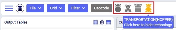
To only show tables and fields in them that can be used by the Hopper transportation optimization algorithm, disable all icons except the 4th (“Transportation”) in the Technologies Selector from the toolbar at the top in Cosmic Frog. This will hide any tables and fields that are not used by Hopper and therefore simplifies the user interface:
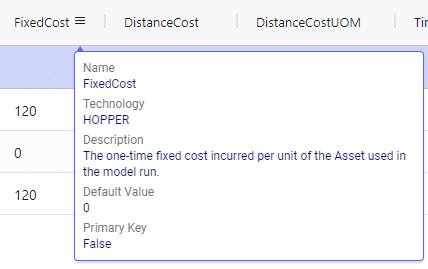
Many Hopper related fields in the input and output tables will be discussed in this document. Keep in mind however that a lot of this information can also be found in the tooltips that are shown when you hover over the column name in a table, see following screenshot for an example. The column name, technology/technologies that use this field, a description of how this field is used by those algorithm(s), its default value, and whether it is part of the table’s primary key are listed in the tooltip.
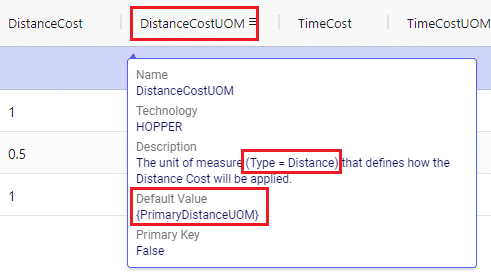
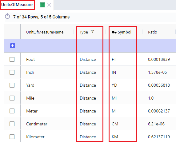
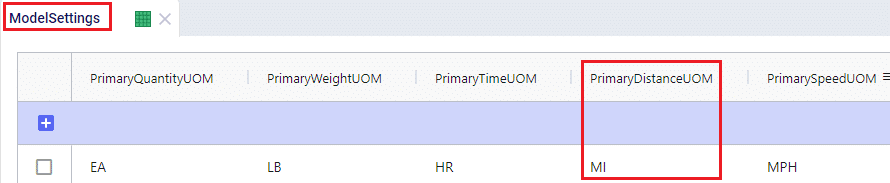
There are a lot of fields with names that end in “…UOM” throughout the input tables. How they work will be explained here so that individual UOM fields across the tables do not need to be explained further in this documentation as they all work similarly. These UOM fields are unit of measure fields and often appear to the immediate right of the field that they apply to, like for example Distance Cost and Distance Cost UOM in the screenshot above. In these UOM fields you can type the Symbol of a unit of measure that is of the required Type from the ones specified in the Units Of Measure table. For example, in the screenshot above, the unit of measure Type for the Distance Cost UOM field is Distance. Looking in the Units of Measure table, we see there are multiple of these specified, like for example Mile (Symbol = MI), Yard (Symbol = YD) and Kilometer (Symbol = KM), so we can use any of these in this UOM field. If we leave a UOM field blank, then the Primary UOM for that UOM Type specified in the Model Settings table will be used. For example, for the Distance Cost UOM field in the screenshot above the tooltip says Default Value = {Primary Distance UOM}. Looking this up in the Model Settings table shows us that this is set to MI (= mile) in our current model. Let’s illustrate this with the following screenshots of 1) the tooltip for the Distance Cost UOM field (located on the Transportation Assets table), 2) units of measure of Type = Distance in the Units Of Measure table and 3) checking what the Primary Distance UOM is set to in the Model Settings table, respectively:
Note that only hours (Symbol = HR) is currently allowed as the Primary Time UOM in the Model Settings table. This means that if another Time UOM, like for example minutes (MIN) or days (DAY), is to be used, the individual UOM fields need to be used to set these. Leaving them blank would mean HR is used by default.
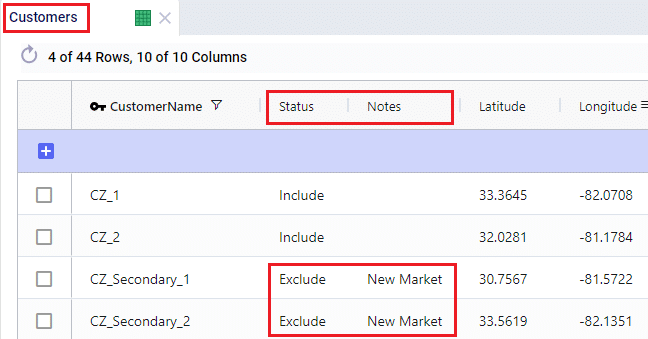
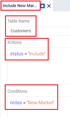
With few exceptions, all tables in Cosmic Frog contain both a Status field and a Notes field. These are often used extensively to add elements to a model that are not currently part of the supply chain (commonly referred to as the “Baseline”), but are to be included in scenarios in case they will definitely become part of the future supply chain or to see whether there are benefits to optionally include these going forward. In these cases, the Status in the input table is set to Exclude and the Notes field often contains a description along the lines of ‘New Market’, ‘New Product’, ‘Box truck for Scenarios 2-4’, ‘Depot for scenario 5’, ‘Include S6’, etc. When creating scenario items for setting up scenarios, the table can then be filtered for Notes = ‘New Market’ while setting Status = ‘Include’ for those filtered records. We will not call out these Status and Notes fields in each individual input table in the remainder of this document, but we definitely do encourage users to use these extensively as they make creating scenarios very easy. When exploring any Cosmic Frog models in the Resource Library, you will notice the extensive use of these fields too. The following 2 screenshots illustrate the use of the Status and Notes fields for scenario creation: 1) shows several customers on the Customers table where CZ_Secondary_1 and CZ_Secondary_2 are not currently customers that are being served but we want to explore what it takes to serve them in future. Their Status is set to Exclude and the Notes field contains ‘New Market’; 2) a scenario item called ‘Include New Market’ shows that the Status of Customers where Notes = ‘New Market’ is changed to ‘Include’.
The Status and Notes fields are also often used for the opposite where existing elements of the current supply chain are excluded in scenarios in cases where for example locations, products or assets are going to go offline in the future. To learn more about scenario creation, please see this short Scenarios Overview video, this Scenario Creation and Maps and Analytics training session video, this Creating Scenarios in Cosmic Frog help article, and this Writing Scenario Syntax help article.
A subset of Cosmic Frog’s input tables needs to be populated in order to run Transportation Optimization, whereas several other tables can be used optionally based on the type of network that is being modelled, and the questions the model needs to answer. The required tables are indicated with a green check mark in the screenshot below, whereas the optional tables have an orange circle in front of them. The Units Of Measure and Model Settings tables are general Cosmic Frog tables, not only used by Hopper and will always be populated with default settings already; these can be added to and changed as needed.

We will first discuss the tables that are required to be populated to set up a basic Hopper model and then cover what can be achieved by also using the optional tables and fields. Note that the screenshots of all input and output tables mostly contain the fields in the order they appear in in the Cosmic Frog user interface, however on occasion the order of the fields was rearranged manually. So, if you do not see a specific field in the same location as in a screenshot, then please scroll through the table to find it.
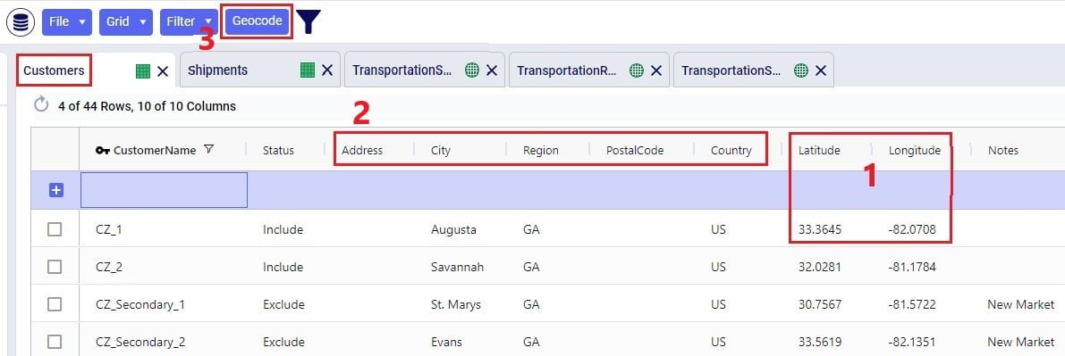
The Customers table contains what for purposes of modelling are considered the customers: the locations that we need to deliver a certain amount of certain product(s) to or pick a certain amount of product(s) up from. The customers need to have their latitudes and longitudes specified so that distances and transport times of route segments can be calculated, and routes can be visualized on a map. Alternatively, users can enter location information like address, city, state, postal code, country and use Cosmic Frog’s built in geocoding tool to populate the latitude and longitude fields. If the customer’s business hours are important to take into account in the Hopper run, its operating schedule can be specified here too, along with customer specific variable and fixed pickup & delivery times. Following screenshot shows an example of several populated records in the Customers table:
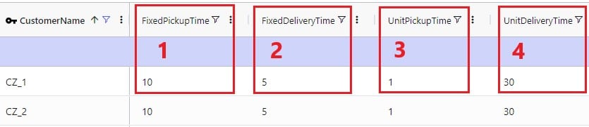
The pickup & delivery time input fields can be seen when scrolling right in the Customers table (the accompanying UOM fields are omitted in this screenshot):
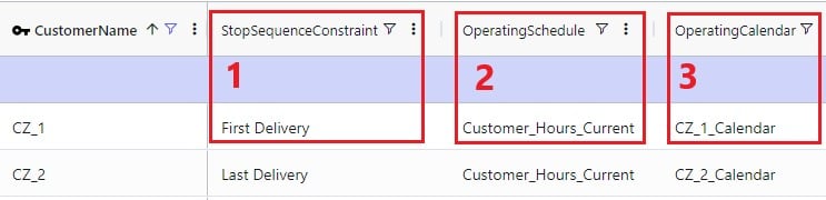
Finally, scrolling even more right, there are 3 additional Hopper-specific fields in the Customers table:
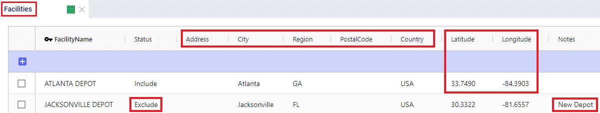
The Facilities table needs to be populated with the location(s) the transportation routes start from and end at; they are the domicile locations for vehicles (assets). The table is otherwise identical to the customers table, where location information can again be used by the geocoding tool to populate the latitude and longitude fields if they are not yet specified. And like other tables, the Status and Notes field are often used to set up scenarios. This screenshot shows the Facilities table populated with 2 depots, 1 current one in Atlanta, GA, and 1 new one in Jacksonville, FL:
Scrolling further right in the Facilities table shows almost all the same fields as those to the right on the Customers table: Operating Schedule, Operating Calendar, and Fixed & Unit Pickup & Delivery Times plus their UOM fields. These all work the same as those on the Customers table, please refer to the descriptions of them in the previous section.
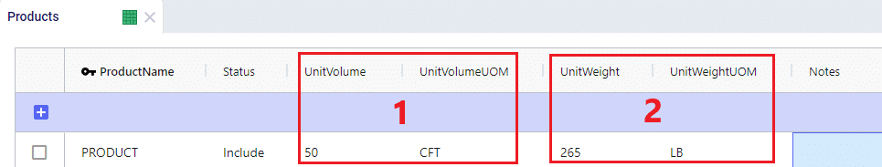
The item(s) that are to be delivered to the customers from the facilities are entered into the Products table. It contains the Product Name, and again a Status and Notes fields for ease of scenario creation. Details around the Volume and Weight of the product are entered here too, which are further explained below this screenshot of the Products table where just one product “PRODUCT” has been specified:
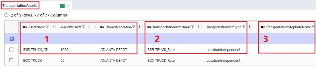
On the Transportation Assets table, the vehicles to be used in the Hopper baseline and any scenario runs are specified. There are a lot of fields around capacities, route and stop details, delivery & pickup times, and driver breaks that can be used on this table, but there is no requirement to use all of them. Use only those that are relevant to your network and the questions you are trying to answer with your model. We will discuss most of them through multiple screenshots. Note that the UOM fields have been omitted in these screenshots. Let’s start with this screenshot showing basic asset details like name, number of units, domicile locations, and rate information:
The following screenshot shows the fields where the operating schedule of the asset, any fixed costs, and capacity of the vehicles can be entered:
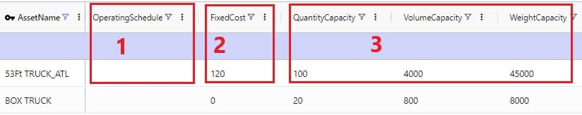
Note that if all 3 of these capacities are specified, the most restrictive one will be used. If you for example know that a certain type of vehicle always cubes out, then you could just populate the Volume Capacity and Volume Capacity UOM fields and leave the other capacity fields blank.
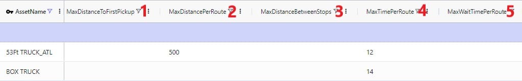
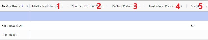
If you scroll further right, you will see the following fields that can be used to set limits on route distance and time when using this type of vehicle. Where applicable, you will notice their UOM fields too (omitted in the screenshot):
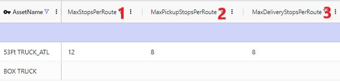
Limits on the amount of stops per route can be set too:
A tour is defined as all the routes a specific unit of a vehicle is used on during the model horizon. Limits around routes, time, and distance for tours can be added if required:
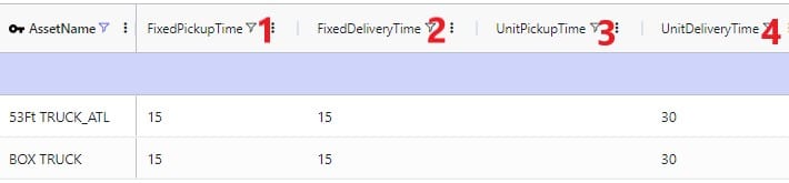
Scrolling still further right you will see the following fields that can be used to add details around how long pickup and delivery take when using this type of vehicle. These all have their own UOM fields too (omitted in the screenshot):
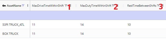
The next 2 screenshots shows the fields on the Transportation Assets table where rules around driver duty, shift, and break times can be entered. Note that these fields each have a UOM field that is not shown in the screenshot:

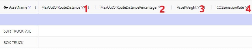
Limits around out of route distance can be set too. Plus details regarding the weight of the asset itself and the level of CO2 emissions:
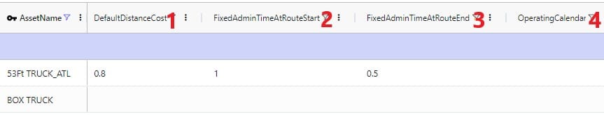
Lastly, a default cost, fixed times for admin, and an operating calendar can be specified for a vehicle in the following fields on the transportation assets table:
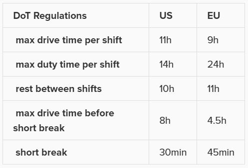
As a reference, these are the department of transportation driver regulations in the US and the EU. They have been somewhat simplified from these sources: US DoT Regulations and EU DoT Regulations:
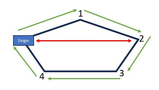
Consider this route that starts from the DC, then goes to CZ1 & CZ2, and then returns to the DC:
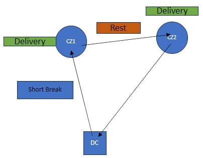
The activities on this route can be thought of as follows, where the start of the Rest is the end of Shift 1 and Shift 2 starts at the end of the Rest:
Notes on Driver Breaks:
Except for asset fixed costs, which are set on the Transportation Assets table, and any Direct Costs which are set on the Shipments table, all costs that can be associated with a multi-stop route can be specified in the Transportation Rates table. The following screenshot shows how a transportation rate is set up with a name, a destination name and the first several cost fields. Note that UOM fields have been omitted in this screenshot, but that each cost field has its own UOM field to specify how the costs should be applied:
Scrolling further right in the Transportation Rates table we see the remaining cost fields:
Finally, a minimum charge and fuel surcharge can be specified as part of a transportation rate too:
The amount of product that needs to be delivered from which source facility/supplier to which destination customer or picked up from which customer is specified on the Shipments table. Optionally, details around pickup and delivery times, direct costs, and fixed template routes can be set on this table too. Note that the Shipments table is Transportation Asset agnostic, meaning that the Hopper transportation optimization algorithm will choose the optimal one to use from the vehicles domiciled at the source location. This first screenshot of the Shipments table shows the basic shipment details:
Here is an example of a subset of Shipments for a model that will route both pickups and deliveries:
To the right in the Shipments table we find the fields where details around shipment windows can be entered:

Still further right on the Shipments table are the fields where details around pickup and delivery times can be specified:
Finally, furthest right on the Shipments table are fields where Direct Costs, details around Template Routes and decompositions can be configured:

Note that there are multiple ways to switching between forcing Shipments and the order of stops onto a template route and letting Hopper optimize which shipments will be put on a route together and in which order. Two example approaches are:
The tables and their input fields that can optionally be populated for their inputs to be used by Hopper will now be covered. Where applicable, it will also be mentioned how Hopper will behave when these are not populated.
In the Transit Matrix table, the transport distance and time for any source-destination-asset combination that could be considered as a segment of a route by Hopper can be specified. Note that the UOM fields in this table are omitted in following screenshot:
The transport distances for any source-destination pairs that are not specified in this table will be calculated based on the latitudes and longitudes of the source and destination and the Circuity Factor that is set in the Model Settings table. Transport times for these pairs will be calculated based on the transport distance and the vehicle’s Speed as set on the Transportation Assets table or, if Speed is not defined on the Transportation Assets table, the Average Speed in the Model Settings table.
Costs that need to be applied on a stop basis can be specified in the Transportation Stop Rates table:
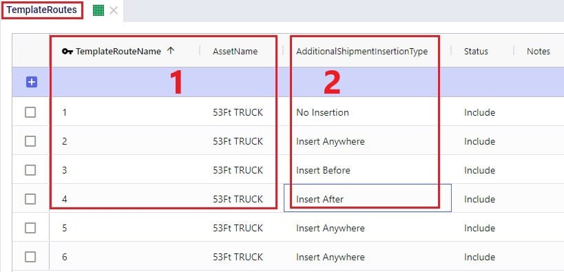
If Template Routes are specified on the Shipments table by using the Template Route Name and Template Route Stop Sequence fields, then the Template Routes table can be used to specify if and how insertions of other Shipments can be made into these template routes:
If a template route is set up by using the Template Route Name and Template Route Stop Sequence fields in the Shipments table and this route is not specified in the Template Routes table, it means that no insertions can be made into this template route.
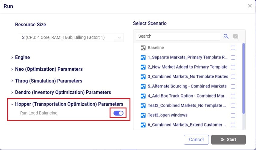
In addition to routing shipments with a fixed amount of product to be delivered to a customer location, Hopper can also solve problems where routes throughout a week need to be designed to balance out weekly demand while achieving the lowest overall routing costs. The Load Balancing Demand and Load Balancing Schedules tables can be used to set this up. If both the Shipments table and the Load Balancing Demand/Schedules tables are populated, by default the Shipments table will be used and the Load Balancing Demand/Schedules tables will be ignored. To switch to using the Load Balancing Demand/Schedules tables (and ignoring the Shipments) table, the Run Load Balancing toggle in the Hopper (Transportation Optimization) Parameters section on the Run screen needs to be switched to on (toggle to the left and grey is off; to the right and blue is on):
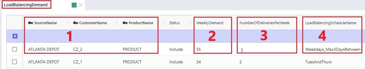
The weekly demand, the number of deliveries per week, and, optionally, a balancing schedule can be specified in the Load Balancing Demand table:
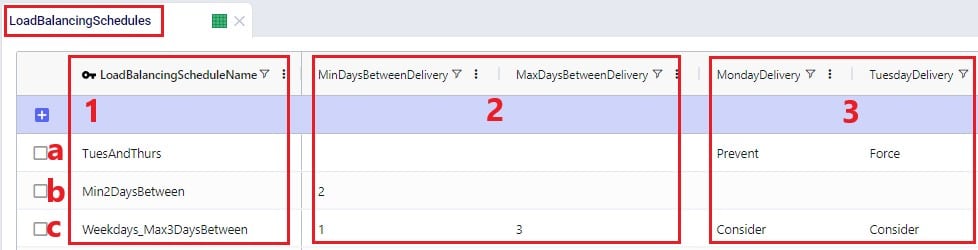
To balance demand over a week according to a schedule, these schedules can be specified in the Load Balancing Schedules table:
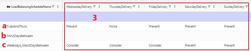
In the screenshots above, the 3 load balancing schedules that have been set up will spread the demand out as follows:
In the Relationship Constraints table, we can tell Hopper what combinations of entities are not allowed on the same route. For example, in the screenshot below we are saying that customers that make up the Primary Market cannot be served on the same route as customers from the Secondary Market:

A few examples of common Relationship Constraints are shown in the following screenshot where the Notes field explains what the constraint does:
To set the availability of customers, facilities, and assets to certain start and end times by day of the week, the Business Hours table can be used. The Schedule Name specified on this table can then be used in the Operating Schedule fields on the Customers, Facilities and Transportation Assets tables. Note that the Wednesday – Saturday Open Time and Close Time fields are omitted in the following screenshot:
To schedule closure of customers, facilities, and assets on certain days, the Business Calendars table can be used. The Calendar Name specified on this table can then be used in the Operating Calendar fields on the Customers, Facilities and Transportation Assets tables:
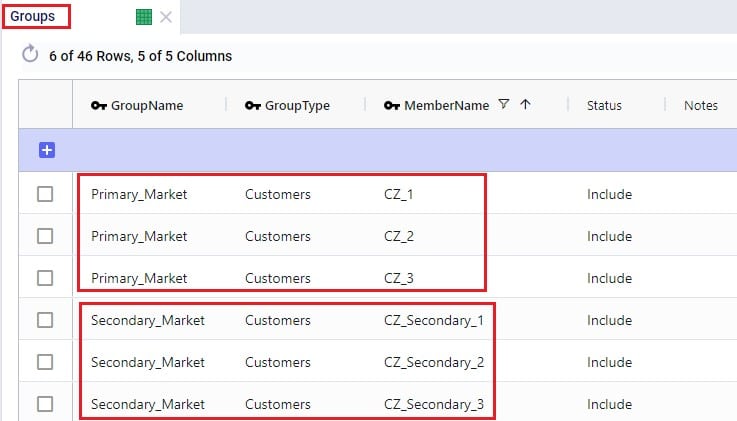
Groups are a general Cosmic Frog feature to make modelling quicker and easier. By grouping elements that behave the same together in a group we can reduce the number of records we need to populate in certain tables since we can use the Group names to populate the fields instead of setting up multiple records for each individual element which will all have the same information otherwise. Underneath the hood, when a model that uses Groups is run, these Groups are enumerated into the individual members of the group. We have for example already seen that groups of Type = Customers were used in the Relationship Constraints table in the previous section to prevent customers in the Primary Market being served on the same route as customers in the Secondary Market. Looking in the Groups table we can see which customers are part (‘members’) of each of these groups:
Examples of other Hopper input tables where use of Groups can be convenient are:
Note that in addition to Groups, Named Filters can be used in these instances too. Learn more about Named Filters in this help center article.
The Step Costs table is a general table in Cosmic Frog used by multiple technologies. It is used to specify costs that change based on the throughput level. For Hopper, all cost fields on the Transportation Rates table, the Transportation Stop Rates table, and the Fixed Cost on the Transportation Assets table can be set up to use Step Costs. We will go through an example of how Step Costs are set up, associated with the correct cost field, and how to understand outputs using the following 3 screenshots of the Step Costs table, Transportation Rates table and Transportation Route Summary output table, respectively. The latter will also be discussed in more detail in the next section on Hopper outputs.

In this example, the per unit cost for units 0 through 20 is $1, $0.9 for units 21 through 40, and $0.85 for all units over 40. Had the Step Cost Behavior field been set to All Item, then the per unit cost for all items is $1 if the throughput is between 0 and 20 units, the per unit cost for all items is $0.9 if the throughput is between 21 and 40 units, and the per unit cost for all items is $0.85 if the throughput is over 41 units.
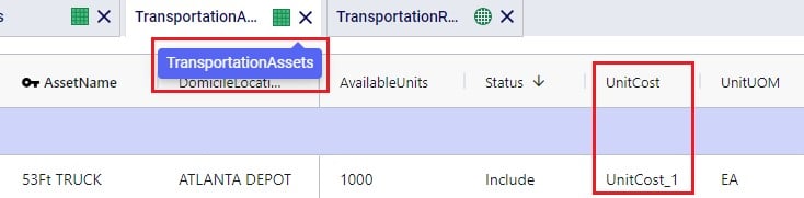
In this screenshot of the Transportation Rates table, it is shown that the Unit Cost field is set to UnitCost_1 which is the stepped cost with 3 throughput levels that we just discussed in the screenshot above:
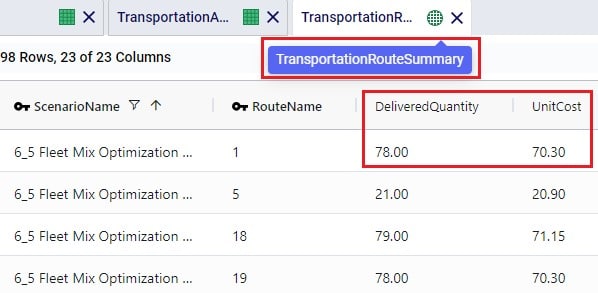
Lastly, this is a screenshot of the Transportation Route Summary output table where we see that the Delivered Quantity on Route 1 is 78. With the stepped cost structure as explained above for UnitCost_1, the Unit Cost in the output is calculated as follows: 20 * $1 (for units 1-20) + 20 * $0.9 (for units 21-40) + 38 * $0.85 (for units 41-78) = $20 + $18 + $32.30 = $70.30.
When the input tables have been populated and scenarios are created (several resources explaining how to set up and configure scenarios are listed in the “2.4 Status and Notes fields” section further above), one can start a Hopper run by clicking on the Run button at the top right in Cosmic Frog:

The Run screen will come up:

Once a Hopper run is completed, the Hopper output tables will contain the outputs of the run.
As with other Cosmic Frog algorithms, we can look at Hopper outputs in output tables, on maps and analytics dashboards. We will discuss each of these in the next 3 sections. Often scenarios will be compared to each other in the outputs to determine which changes need to be made to the last-mile delivery part of the supply chain.
In the Output Summary Tables section of the Output Tables are 8 Hopper specific tables, they start with “Transportation…”. Plus, there is also the Hopper specific detailed Transportation Activity Report table in the Output Report Tables section:
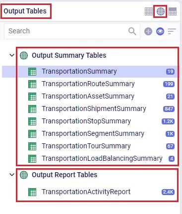
Switch from viewing Input Tables to Output Tables by clicking on the round grid at the top right of the tables list. The Transportation Summary table gives a high-level summary of each Hopper scenario that has been run and the next 6 Summary output tables contain the detailed outputs at the route, asset, shipment, stop, segment, and tour level. The Transportation Load Balancing Summary output table is populated when a Load Balancing scenario has been run, and summarizes outputs at the daily level. The Transportation Activity Report is especially useful to understand when Rests and Breaks are required on a route. All these output tables will be covered individually in the following sections.
The Transportation Summary table contains outputs for each scenario run that include Hopper run details, cost details, how much product was delivered and how, total distance and time, and how many routes, stops and shipments there were in total.
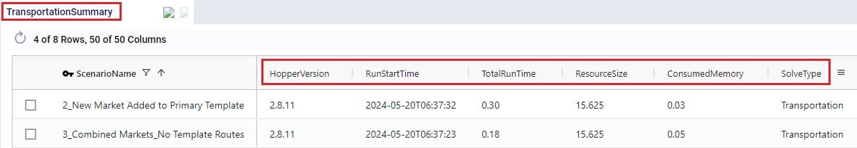
The Hopper run details that are listed for each scenario include:
The next 2 screenshots show the Hopper cost outputs, summarized by scenario:


Scrolling further right in the Transportation Summary table shows the details around how much product was delivered in each scenario:
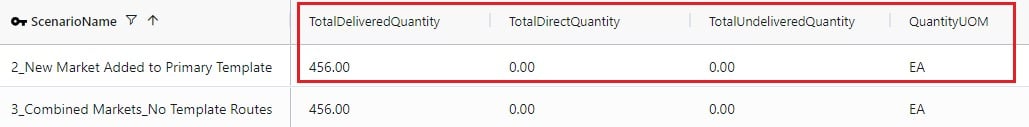
For the Quantity UOM that is shown in the farthest right column in this screenshot (eaches here), the Total Delivered Quantity, Total Direct Quantity and Total Undelivered Quantity are listed in these columns. If the Total Direct Quantity is greater than 0, details around which shipments were delivered directly to the customer can be found in the Transportation Shipment Summary output table where the Shipment Status = Direct Shipping. Similarly, if the total undelivered quantity is greater than 0, then more details on which shipments were not delivered and why are detailed in the Unrouted Reason field of the Transportation Shipment Summary output table where the Shipment Status = Unrouted.
The next set of output columns when scrolling further right repeat these delivered, direct and undelivered amounts by scenario, but in terms of volume and weight.
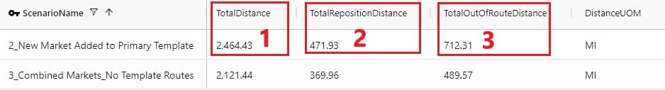
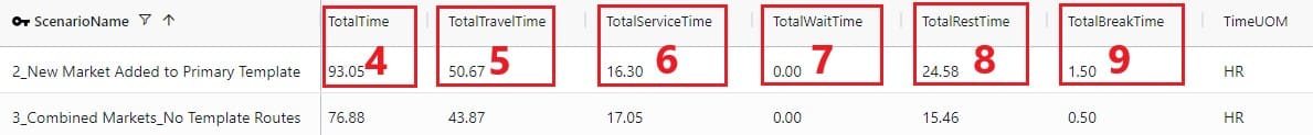
Still further to the right we find the outputs that summarize the total distance and time by scenario:
Lastly, the fields furthest right on the Transportation Summary output table contain details around the number of routes, assets and shipments, and CO2 emissions:

A few columns contained in this table are not shown in any of the above screenshots, these are:
The Transportation Route Summary table contains details for each route in each scenario that include cost, distance & time, number of stops & shipments, and the amount of product delivered on the route.
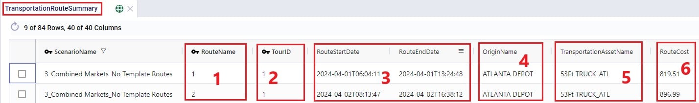
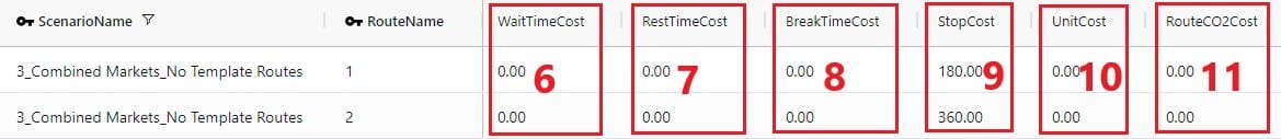
The costs that together make up the total Route Cost are listed in the next 11 fields shown in the next 2 screenshots:

The next set of output fields show the distance and time for each route:
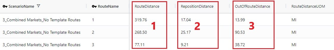

Finally, the fields furthest right in the Transportation Route Summary table list the amount of product that was delivered on the routes, and the number of stops and delivered shipments on each route.

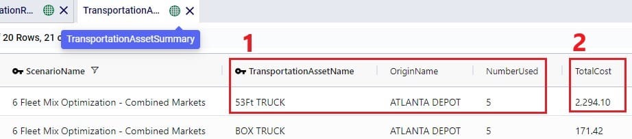
The Transportation Asset Summary output table contains the details of each type of asset used in each scenario. These details include costs, amount of product delivered, distance & time, and the number of delivered shipments.
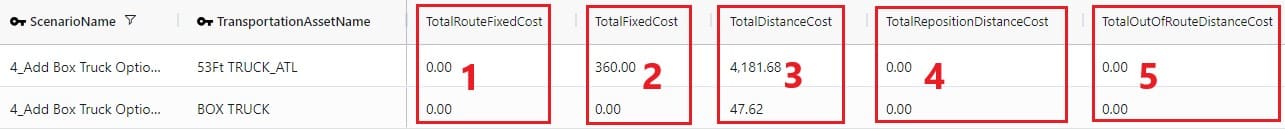
The costs that together make up the Total Cost are listed in the next 12 fields:

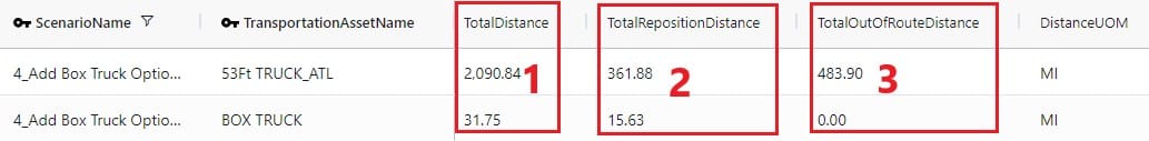
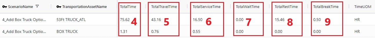
The next set of fields in the Transportation Asset Summary summarize the distances and times by asset type for the scenario:
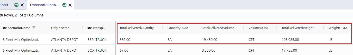
Furthest to the right on the Transportation Asset Summary output table we find the outputs that list the total amount of product that was delivered, the number of delivered shipments, and the total CO2 emissions:
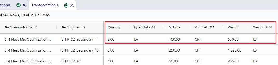
The Transportation Shipment Summary output table lists for each included Shipment of the scenario the details of which asset type it is served by, which stop on which route it is, the amount of product delivered, the allocated cost, and its status.

The next set of fields in the Transportation Shipment Summary table list the total amount of product that was delivered to this stop.
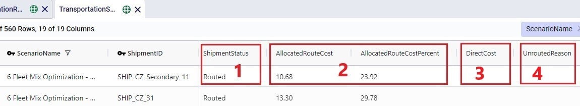
The next screenshot of the Transportation Shipment Summary shows the outputs that detail the status of the shipment, costs, and a reason in case the shipment was unrouted.
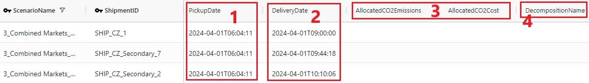
Lastly, the outputs furthest to the right on the Transportation Shipment Summary output table list the pickup and delivery time and dates, the allocation of CO2 emissions and associated costs, and the Decomposition Name if used:
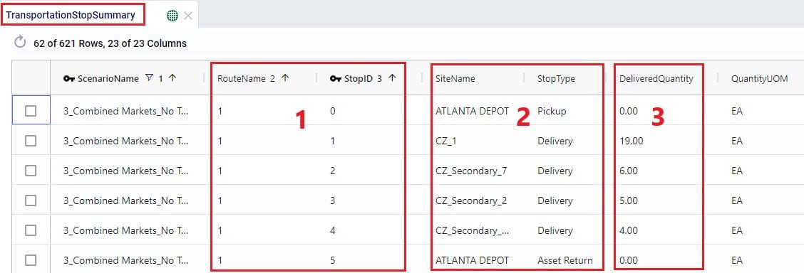
The Transportation Stop Summary output table lists for each route all the individual stops and their details around amount of product delivered, allocated cost, service time, and stop location information.
This first screenshot shows the basic details of the stops in terms of route name, stop ID, location, stop type, and how much product was delivered:
Somewhat further right on the Transportation Stop Summary table we find the outputs that detail the route cost allocation and the different types of time spent at the stop:
Lastly, farthest right on the Transportation Stop Summary table, arrival, service, and departure dates are listed, along with the stop’s latitude and longitude:
The Transportation Segment Summary output table contains distance, time, and source and destination location details for each segment (or “leg”) of each route.
The basic details of each segment are shown in the following screenshot of the Transportation Segment Summary table:
Further right on the Transportation Segment Summary output table, the time details of each segment are shown:

Next on the Transportation Segment Summary table are the latitudes and longitudes of the segment’s origin and destination locations:
And farthest right on the Transportation Segment Summary output table details around the start and end date and time of the segment are listed, plus CO2 emissions and the associated CO2 cost:

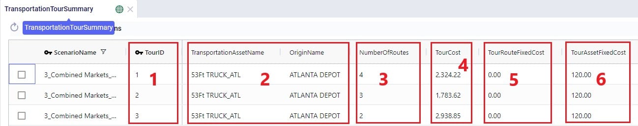
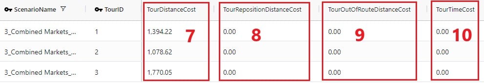
For each Tour (= asset schedule) the Transportation Tour Summary output table summarizes the costs, distances, times, and CO2 details.
The next 3 screenshots show the basic tour details and all costs associated with a tour:

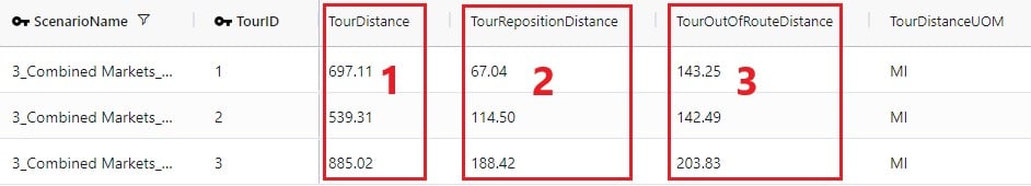
The next screenshot shows the distance outputs available for each tour on the Transportation Tour Summary output table:
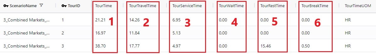
Scrolling further right on the Transportation Tour Summary table, the outputs available for tour times are listed:

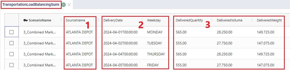
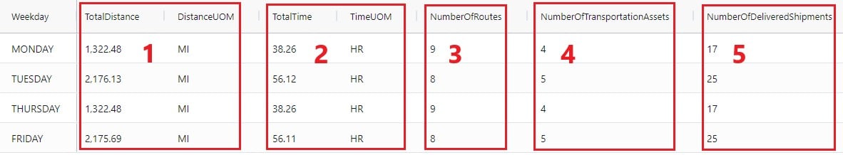
If a load balancing scenario has been run (see the Load Balancing Demand input table further above for more details on how to run this), then the Transportation Load Balancing Summary output table will be populated too. Details on amount of product delivered, plus the number of routes, assets and delivered shipments by day of the week can be found in this output table; see the following 2 screenshots:
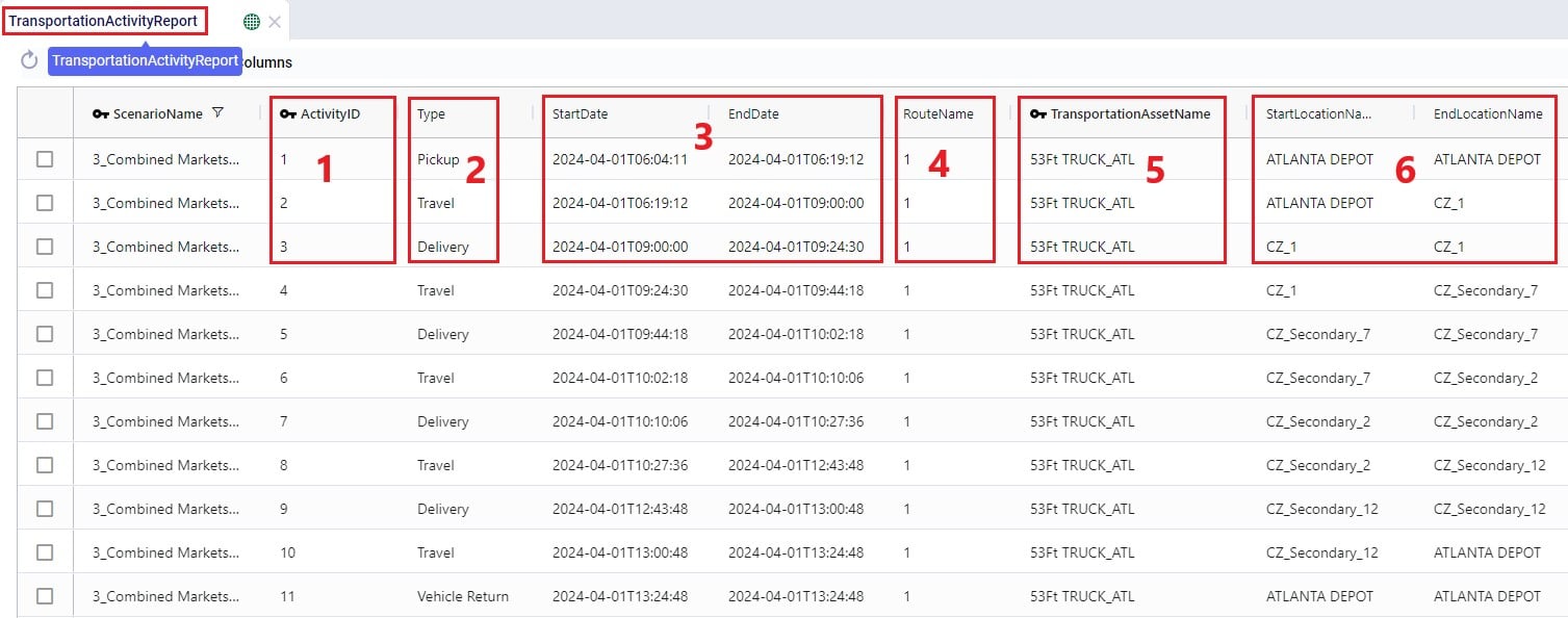
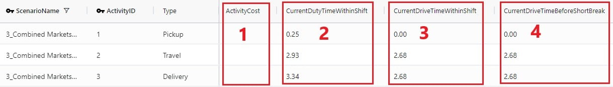
For each route, the Transportation Activity Report details all the activities that happen in chronological order with details around distance and time and it breaks down how far along the duty and drive times are at each point in the route, which is very helpful to understand when rests and short breaks are happening.
This first screenshot of the Transportation Activity Report shows the basic details of the activities:
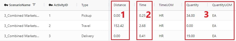
Next, the distance, time, and delivered amount of product are detailed on the Transportation Activity Report:
Finally, the last several fields on the Transportation Activity Report details cost, and the thus far accumulated duty and drive times:
As with the other engines within Cosmic Frog, Maps are very helpful in visualizing baseline and scenario outputs. Here, we will discuss how to set up Hopper specific Maps at a high level; we will not cover all the ins and outs of maps. If you are unfamiliar with the Maps module in Cosmic Frog, then please review the “Getting Started with Maps” article in the Optilogic Help Center first. It covers how to add and configure new maps and their layers.
Visualizing Hopper routes and direct shipments on maps is achieved by adding map layers which use 1 of the following as the table name:
Using what we have discussed above and the learnings from the Getting Started with Maps help center article, we can create the following map quite easily and quickly (the model used here is one from the Resource Library, named Transportation Optimization):
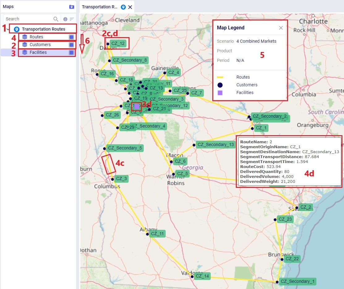
The steps taken to create this map are:
Let’s also cover 2 maps of a model where both pickups and deliveries are being made, from “backhaul” and to “linehaul” customers, respectively. When setting the LIFO (Is Last In First Out) field on the Transportation Assets table to True, this leads to routes that contain both pickup and delivery stops, but all the pickups are made at the end (e.g. modeling backhaul):
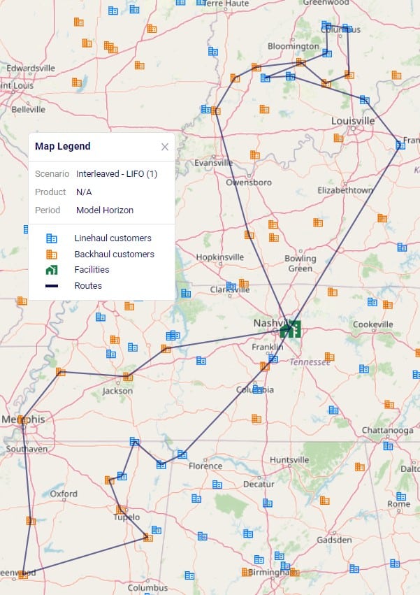
Two example routes are being shown in the screenshot above and we can see that all deliveries are first made to the linehaul customers which have blue icons. Then, pickups are made at the backhaul customers which have orange icons. If we want to design interleaved routes where pickups and deliveries can be mixed, we need to set the LIFO field to False. The following screenshot shows 2 of these interleaved routes:

The above 2 screenshots use the Transportation Routes Map Layer as the table name to draw the Routes map layer, where the condition builder is used to filter for 2 of the route names.
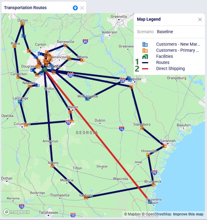
Finally, we will go back to the Transportation Optimization model which was used for the first map screenshot in this section. The Baseline scenario in this model has 1 shipment that is being shipped directly. To visualize this on the map we add a map layer named "Direct Shipping" which uses the Transportation Shipment Summary as the table name input. On the Layer Style pane we change the color for this line layer to red. We also keep the "Routes" map layer, which is drawn from the Transportation Routes Map Layer with the default dark blue color:
In the Analytics module of Cosmic Frog, dashboards that show graphs of scenario outputs, sliced and diced to the user’s preferences, can quickly be configured. Like Maps, this functionality is not Hopper specific and other Cosmic Frog technologies use these extensively too. We will cover setting up a Hopper specific visualization, but not all the details of configuring dashboards. Please review these resources on Analytics in Cosmic Frog first if you are not yet familiar with these:
We will do a quick step by step walk through of how to set up a visualization of comparing scenario costs by cost type in a new dashboard:
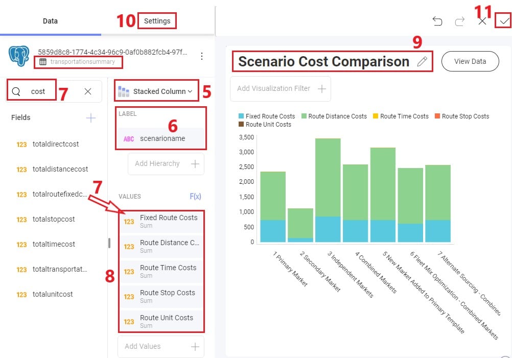
The steps to set this up are detailed here, note that the first 4 bullet points are not shown in the screenshot above:
There are several models in the Resource Library that transportation optimization users may find helpful to review. How to use resources in the Resource Library is described in the help center article “How to Use the Resource Library”.
Hopper is the Transportation Optimization algorithm within Cosmic Frog. It designs optimal multi-stop routes to deliver/pickup a given set of shipments to/from customer locations at the lowest cost. Fleet sizing and balancing weekly demand can be achieved with Hopper too. Example business questions Hopper can answer are:
Hopper’s transportation optimization capabilities can be used in combination with network design to test out what a new network design means in terms of the last-mile delivery configuration. For example, questions that can be looked at are:
With ever increasing transportation costs, getting the last-mile delivery part of your supply chain right can make a big impact on the overall supply chain costs!
It is recommended to watch this short Getting Started with Hopper video before diving into the details of this documentation. The video gives a nice, concise overview of the basic inputs, process, and outputs of a Hopper model.
In this documentation we will first cover some general Cosmic Frog functionality that is used extensively in Hopper, next we go through how to build a Hopper model which discusses required and optional inputs, how to run a Hopper model is explained, Hopper outputs in tables, on maps and analytics are covered as well, and finally references to a few additional Hopper resources are listed. Note that the use of user-defined variables, costs and constraints for Hopper models is covered in a separate help article.
To not make this document too repetitive we will cover some general Cosmic Frog functionality here that applies to all Cosmic Frog technologies and is used extensively for Hopper too.
To only show tables and fields in them that can be used by the Hopper transportation optimization algorithm, disable all icons except the 4th (“Transportation”) in the Technologies Selector from the toolbar at the top in Cosmic Frog. This will hide any tables and fields that are not used by Hopper and therefore simplifies the user interface:
Many Hopper related fields in the input and output tables will be discussed in this document. Keep in mind however that a lot of this information can also be found in the tooltips that are shown when you hover over the column name in a table, see following screenshot for an example. The column name, technology/technologies that use this field, a description of how this field is used by those algorithm(s), its default value, and whether it is part of the table’s primary key are listed in the tooltip.
There are a lot of fields with names that end in “…UOM” throughout the input tables. How they work will be explained here so that individual UOM fields across the tables do not need to be explained further in this documentation as they all work similarly. These UOM fields are unit of measure fields and often appear to the immediate right of the field that they apply to, like for example Distance Cost and Distance Cost UOM in the screenshot above. In these UOM fields you can type the Symbol of a unit of measure that is of the required Type from the ones specified in the Units Of Measure table. For example, in the screenshot above, the unit of measure Type for the Distance Cost UOM field is Distance. Looking in the Units of Measure table, we see there are multiple of these specified, like for example Mile (Symbol = MI), Yard (Symbol = YD) and Kilometer (Symbol = KM), so we can use any of these in this UOM field. If we leave a UOM field blank, then the Primary UOM for that UOM Type specified in the Model Settings table will be used. For example, for the Distance Cost UOM field in the screenshot above the tooltip says Default Value = {Primary Distance UOM}. Looking this up in the Model Settings table shows us that this is set to MI (= mile) in our current model. Let’s illustrate this with the following screenshots of 1) the tooltip for the Distance Cost UOM field (located on the Transportation Assets table), 2) units of measure of Type = Distance in the Units Of Measure table and 3) checking what the Primary Distance UOM is set to in the Model Settings table, respectively:
Note that only hours (Symbol = HR) is currently allowed as the Primary Time UOM in the Model Settings table. This means that if another Time UOM, like for example minutes (MIN) or days (DAY), is to be used, the individual UOM fields need to be used to set these. Leaving them blank would mean HR is used by default.
With few exceptions, all tables in Cosmic Frog contain both a Status field and a Notes field. These are often used extensively to add elements to a model that are not currently part of the supply chain (commonly referred to as the “Baseline”), but are to be included in scenarios in case they will definitely become part of the future supply chain or to see whether there are benefits to optionally include these going forward. In these cases, the Status in the input table is set to Exclude and the Notes field often contains a description along the lines of ‘New Market’, ‘New Product’, ‘Box truck for Scenarios 2-4’, ‘Depot for scenario 5’, ‘Include S6’, etc. When creating scenario items for setting up scenarios, the table can then be filtered for Notes = ‘New Market’ while setting Status = ‘Include’ for those filtered records. We will not call out these Status and Notes fields in each individual input table in the remainder of this document, but we definitely do encourage users to use these extensively as they make creating scenarios very easy. When exploring any Cosmic Frog models in the Resource Library, you will notice the extensive use of these fields too. The following 2 screenshots illustrate the use of the Status and Notes fields for scenario creation: 1) shows several customers on the Customers table where CZ_Secondary_1 and CZ_Secondary_2 are not currently customers that are being served but we want to explore what it takes to serve them in future. Their Status is set to Exclude and the Notes field contains ‘New Market’; 2) a scenario item called ‘Include New Market’ shows that the Status of Customers where Notes = ‘New Market’ is changed to ‘Include’.
The Status and Notes fields are also often used for the opposite where existing elements of the current supply chain are excluded in scenarios in cases where for example locations, products or assets are going to go offline in the future. To learn more about scenario creation, please see this short Scenarios Overview video, this Scenario Creation and Maps and Analytics training session video, this Creating Scenarios in Cosmic Frog help article, and this Writing Scenario Syntax help article.
A subset of Cosmic Frog’s input tables needs to be populated in order to run Transportation Optimization, whereas several other tables can be used optionally based on the type of network that is being modelled, and the questions the model needs to answer. The required tables are indicated with a green check mark in the screenshot below, whereas the optional tables have an orange circle in front of them. The Units Of Measure and Model Settings tables are general Cosmic Frog tables, not only used by Hopper and will always be populated with default settings already; these can be added to and changed as needed.
We will first discuss the tables that are required to be populated to set up a basic Hopper model and then cover what can be achieved by also using the optional tables and fields. Note that the screenshots of all input and output tables mostly contain the fields in the order they appear in in the Cosmic Frog user interface, however on occasion the order of the fields was rearranged manually. So, if you do not see a specific field in the same location as in a screenshot, then please scroll through the table to find it.
The Customers table contains what for purposes of modelling are considered the customers: the locations that we need to deliver a certain amount of certain product(s) to or pick a certain amount of product(s) up from. The customers need to have their latitudes and longitudes specified so that distances and transport times of route segments can be calculated, and routes can be visualized on a map. Alternatively, users can enter location information like address, city, state, postal code, country and use Cosmic Frog’s built in geocoding tool to populate the latitude and longitude fields. If the customer’s business hours are important to take into account in the Hopper run, its operating schedule can be specified here too, along with customer specific variable and fixed pickup & delivery times. Following screenshot shows an example of several populated records in the Customers table:
The pickup & delivery time input fields can be seen when scrolling right in the Customers table (the accompanying UOM fields are omitted in this screenshot):
Finally, scrolling even more right, there are 3 additional Hopper-specific fields in the Customers table:
The Facilities table needs to be populated with the location(s) the transportation routes start from and end at; they are the domicile locations for vehicles (assets). The table is otherwise identical to the customers table, where location information can again be used by the geocoding tool to populate the latitude and longitude fields if they are not yet specified. And like other tables, the Status and Notes field are often used to set up scenarios. This screenshot shows the Facilities table populated with 2 depots, 1 current one in Atlanta, GA, and 1 new one in Jacksonville, FL:
Scrolling further right in the Facilities table shows almost all the same fields as those to the right on the Customers table: Operating Schedule, Operating Calendar, and Fixed & Unit Pickup & Delivery Times plus their UOM fields. These all work the same as those on the Customers table, please refer to the descriptions of them in the previous section.
The item(s) that are to be delivered to the customers from the facilities are entered into the Products table. It contains the Product Name, and again a Status and Notes fields for ease of scenario creation. Details around the Volume and Weight of the product are entered here too, which are further explained below this screenshot of the Products table where just one product “PRODUCT” has been specified:
On the Transportation Assets table, the vehicles to be used in the Hopper baseline and any scenario runs are specified. There are a lot of fields around capacities, route and stop details, delivery & pickup times, and driver breaks that can be used on this table, but there is no requirement to use all of them. Use only those that are relevant to your network and the questions you are trying to answer with your model. We will discuss most of them through multiple screenshots. Note that the UOM fields have been omitted in these screenshots. Let’s start with this screenshot showing basic asset details like name, number of units, domicile locations, and rate information:
The following screenshot shows the fields where the operating schedule of the asset, any fixed costs, and capacity of the vehicles can be entered:
Note that if all 3 of these capacities are specified, the most restrictive one will be used. If you for example know that a certain type of vehicle always cubes out, then you could just populate the Volume Capacity and Volume Capacity UOM fields and leave the other capacity fields blank.
If you scroll further right, you will see the following fields that can be used to set limits on route distance and time when using this type of vehicle. Where applicable, you will notice their UOM fields too (omitted in the screenshot):
Limits on the amount of stops per route can be set too:
A tour is defined as all the routes a specific unit of a vehicle is used on during the model horizon. Limits around routes, time, and distance for tours can be added if required:
Scrolling still further right you will see the following fields that can be used to add details around how long pickup and delivery take when using this type of vehicle. These all have their own UOM fields too (omitted in the screenshot):
The next 2 screenshots shows the fields on the Transportation Assets table where rules around driver duty, shift, and break times can be entered. Note that these fields each have a UOM field that is not shown in the screenshot:
Limits around out of route distance can be set too. Plus details regarding the weight of the asset itself and the level of CO2 emissions:
Lastly, a default cost, fixed times for admin, and an operating calendar can be specified for a vehicle in the following fields on the transportation assets table:
As a reference, these are the department of transportation driver regulations in the US and the EU. They have been somewhat simplified from these sources: US DoT Regulations and EU DoT Regulations:
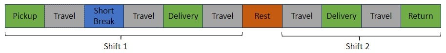
Consider this route that starts from the DC, then goes to CZ1 & CZ2, and then returns to the DC:
The activities on this route can be thought of as follows, where the start of the Rest is the end of Shift 1 and Shift 2 starts at the end of the Rest:
Notes on Driver Breaks:
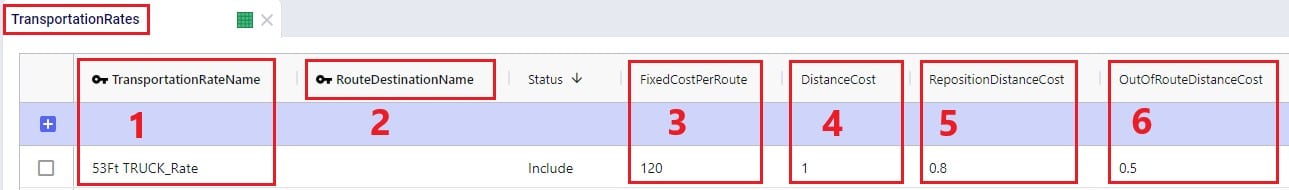
Except for asset fixed costs, which are set on the Transportation Assets table, and any Direct Costs which are set on the Shipments table, all costs that can be associated with a multi-stop route can be specified in the Transportation Rates table. The following screenshot shows how a transportation rate is set up with a name, a destination name and the first several cost fields. Note that UOM fields have been omitted in this screenshot, but that each cost field has its own UOM field to specify how the costs should be applied:
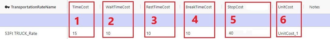
Scrolling further right in the Transportation Rates table we see the remaining cost fields:
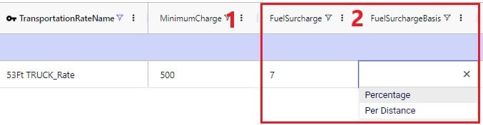
Finally, a minimum charge and fuel surcharge can be specified as part of a transportation rate too:
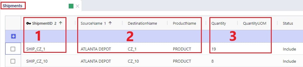
The amount of product that needs to be delivered from which source facility/supplier to which destination customer or picked up from which customer is specified on the Shipments table. Optionally, details around pickup and delivery times, direct costs, and fixed template routes can be set on this table too. Note that the Shipments table is Transportation Asset agnostic, meaning that the Hopper transportation optimization algorithm will choose the optimal one to use from the vehicles domiciled at the source location. This first screenshot of the Shipments table shows the basic shipment details:
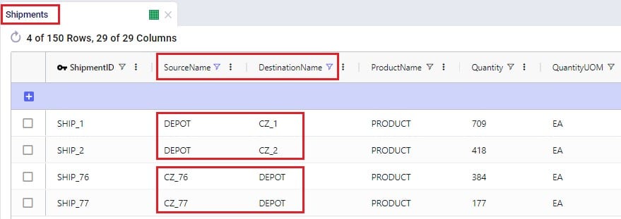
Here is an example of a subset of Shipments for a model that will route both pickups and deliveries:
To the right in the Shipments table we find the fields where details around shipment windows can be entered:
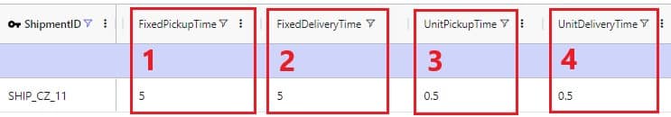
Still further right on the Shipments table are the fields where details around pickup and delivery times can be specified:
Finally, furthest right on the Shipments table are fields where Direct Costs, details around Template Routes and decompositions can be configured:
Note that there are multiple ways to switching between forcing Shipments and the order of stops onto a template route and letting Hopper optimize which shipments will be put on a route together and in which order. Two example approaches are:
The tables and their input fields that can optionally be populated for their inputs to be used by Hopper will now be covered. Where applicable, it will also be mentioned how Hopper will behave when these are not populated.
In the Transit Matrix table, the transport distance and time for any source-destination-asset combination that could be considered as a segment of a route by Hopper can be specified. Note that the UOM fields in this table are omitted in following screenshot:
The transport distances for any source-destination pairs that are not specified in this table will be calculated based on the latitudes and longitudes of the source and destination and the Circuity Factor that is set in the Model Settings table. Transport times for these pairs will be calculated based on the transport distance and the vehicle’s Speed as set on the Transportation Assets table or, if Speed is not defined on the Transportation Assets table, the Average Speed in the Model Settings table.
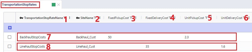
Costs that need to be applied on a stop basis can be specified in the Transportation Stop Rates table:
If Template Routes are specified on the Shipments table by using the Template Route Name and Template Route Stop Sequence fields, then the Template Routes table can be used to specify if and how insertions of other Shipments can be made into these template routes:
If a template route is set up by using the Template Route Name and Template Route Stop Sequence fields in the Shipments table and this route is not specified in the Template Routes table, it means that no insertions can be made into this template route.
In addition to routing shipments with a fixed amount of product to be delivered to a customer location, Hopper can also solve problems where routes throughout a week need to be designed to balance out weekly demand while achieving the lowest overall routing costs. The Load Balancing Demand and Load Balancing Schedules tables can be used to set this up. If both the Shipments table and the Load Balancing Demand/Schedules tables are populated, by default the Shipments table will be used and the Load Balancing Demand/Schedules tables will be ignored. To switch to using the Load Balancing Demand/Schedules tables (and ignoring the Shipments) table, the Run Load Balancing toggle in the Hopper (Transportation Optimization) Parameters section on the Run screen needs to be switched to on (toggle to the left and grey is off; to the right and blue is on):
The weekly demand, the number of deliveries per week, and, optionally, a balancing schedule can be specified in the Load Balancing Demand table:
To balance demand over a week according to a schedule, these schedules can be specified in the Load Balancing Schedules table:
In the screenshots above, the 3 load balancing schedules that have been set up will spread the demand out as follows:
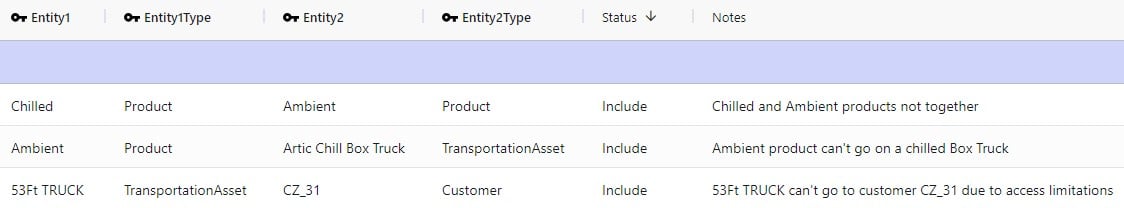
In the Relationship Constraints table, we can tell Hopper what combinations of entities are not allowed on the same route. For example, in the screenshot below we are saying that customers that make up the Primary Market cannot be served on the same route as customers from the Secondary Market:
A few examples of common Relationship Constraints are shown in the following screenshot where the Notes field explains what the constraint does:
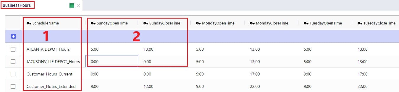
To set the availability of customers, facilities, and assets to certain start and end times by day of the week, the Business Hours table can be used. The Schedule Name specified on this table can then be used in the Operating Schedule fields on the Customers, Facilities and Transportation Assets tables. Note that the Wednesday – Saturday Open Time and Close Time fields are omitted in the following screenshot:
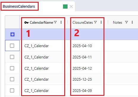
To schedule closure of customers, facilities, and assets on certain days, the Business Calendars table can be used. The Calendar Name specified on this table can then be used in the Operating Calendar fields on the Customers, Facilities and Transportation Assets tables:
Groups are a general Cosmic Frog feature to make modelling quicker and easier. By grouping elements that behave the same together in a group we can reduce the number of records we need to populate in certain tables since we can use the Group names to populate the fields instead of setting up multiple records for each individual element which will all have the same information otherwise. Underneath the hood, when a model that uses Groups is run, these Groups are enumerated into the individual members of the group. We have for example already seen that groups of Type = Customers were used in the Relationship Constraints table in the previous section to prevent customers in the Primary Market being served on the same route as customers in the Secondary Market. Looking in the Groups table we can see which customers are part (‘members’) of each of these groups:
Examples of other Hopper input tables where use of Groups can be convenient are:
Note that in addition to Groups, Named Filters can be used in these instances too. Learn more about Named Filters in this help center article.
The Step Costs table is a general table in Cosmic Frog used by multiple technologies. It is used to specify costs that change based on the throughput level. For Hopper, all cost fields on the Transportation Rates table, the Transportation Stop Rates table, and the Fixed Cost on the Transportation Assets table can be set up to use Step Costs. We will go through an example of how Step Costs are set up, associated with the correct cost field, and how to understand outputs using the following 3 screenshots of the Step Costs table, Transportation Rates table and Transportation Route Summary output table, respectively. The latter will also be discussed in more detail in the next section on Hopper outputs.
In this example, the per unit cost for units 0 through 20 is $1, $0.9 for units 21 through 40, and $0.85 for all units over 40. Had the Step Cost Behavior field been set to All Item, then the per unit cost for all items is $1 if the throughput is between 0 and 20 units, the per unit cost for all items is $0.9 if the throughput is between 21 and 40 units, and the per unit cost for all items is $0.85 if the throughput is over 41 units.
In this screenshot of the Transportation Rates table, it is shown that the Unit Cost field is set to UnitCost_1 which is the stepped cost with 3 throughput levels that we just discussed in the screenshot above:
Lastly, this is a screenshot of the Transportation Route Summary output table where we see that the Delivered Quantity on Route 1 is 78. With the stepped cost structure as explained above for UnitCost_1, the Unit Cost in the output is calculated as follows: 20 * $1 (for units 1-20) + 20 * $0.9 (for units 21-40) + 38 * $0.85 (for units 41-78) = $20 + $18 + $32.30 = $70.30.
When the input tables have been populated and scenarios are created (several resources explaining how to set up and configure scenarios are listed in the “2.4 Status and Notes fields” section further above), one can start a Hopper run by clicking on the Run button at the top right in Cosmic Frog:
The Run screen will come up:
Once a Hopper run is completed, the Hopper output tables will contain the outputs of the run.
As with other Cosmic Frog algorithms, we can look at Hopper outputs in output tables, on maps and analytics dashboards. We will discuss each of these in the next 3 sections. Often scenarios will be compared to each other in the outputs to determine which changes need to be made to the last-mile delivery part of the supply chain.
In the Output Summary Tables section of the Output Tables are 8 Hopper specific tables, they start with “Transportation…”. Plus, there is also the Hopper specific detailed Transportation Activity Report table in the Output Report Tables section:
Switch from viewing Input Tables to Output Tables by clicking on the round grid at the top right of the tables list. The Transportation Summary table gives a high-level summary of each Hopper scenario that has been run and the next 6 Summary output tables contain the detailed outputs at the route, asset, shipment, stop, segment, and tour level. The Transportation Load Balancing Summary output table is populated when a Load Balancing scenario has been run, and summarizes outputs at the daily level. The Transportation Activity Report is especially useful to understand when Rests and Breaks are required on a route. All these output tables will be covered individually in the following sections.
The Transportation Summary table contains outputs for each scenario run that include Hopper run details, cost details, how much product was delivered and how, total distance and time, and how many routes, stops and shipments there were in total.
The Hopper run details that are listed for each scenario include:
The next 2 screenshots show the Hopper cost outputs, summarized by scenario:
Scrolling further right in the Transportation Summary table shows the details around how much product was delivered in each scenario:
For the Quantity UOM that is shown in the farthest right column in this screenshot (eaches here), the Total Delivered Quantity, Total Direct Quantity and Total Undelivered Quantity are listed in these columns. If the Total Direct Quantity is greater than 0, details around which shipments were delivered directly to the customer can be found in the Transportation Shipment Summary output table where the Shipment Status = Direct Shipping. Similarly, if the total undelivered quantity is greater than 0, then more details on which shipments were not delivered and why are detailed in the Unrouted Reason field of the Transportation Shipment Summary output table where the Shipment Status = Unrouted.
The next set of output columns when scrolling further right repeat these delivered, direct and undelivered amounts by scenario, but in terms of volume and weight.
Still further to the right we find the outputs that summarize the total distance and time by scenario:
Lastly, the fields furthest right on the Transportation Summary output table contain details around the number of routes, assets and shipments, and CO2 emissions:
A few columns contained in this table are not shown in any of the above screenshots, these are:
The Transportation Route Summary table contains details for each route in each scenario that include cost, distance & time, number of stops & shipments, and the amount of product delivered on the route.
The costs that together make up the total Route Cost are listed in the next 11 fields shown in the next 2 screenshots:
The next set of output fields show the distance and time for each route:
Finally, the fields furthest right in the Transportation Route Summary table list the amount of product that was delivered on the routes, and the number of stops and delivered shipments on each route.
The Transportation Asset Summary output table contains the details of each type of asset used in each scenario. These details include costs, amount of product delivered, distance & time, and the number of delivered shipments.
The costs that together make up the Total Cost are listed in the next 12 fields:
The next set of fields in the Transportation Asset Summary summarize the distances and times by asset type for the scenario:
Furthest to the right on the Transportation Asset Summary output table we find the outputs that list the total amount of product that was delivered, the number of delivered shipments, and the total CO2 emissions:
The Transportation Shipment Summary output table lists for each included Shipment of the scenario the details of which asset type it is served by, which stop on which route it is, the amount of product delivered, the allocated cost, and its status.
The next set of fields in the Transportation Shipment Summary table list the total amount of product that was delivered to this stop.
The next screenshot of the Transportation Shipment Summary shows the outputs that detail the status of the shipment, costs, and a reason in case the shipment was unrouted.
Lastly, the outputs furthest to the right on the Transportation Shipment Summary output table list the pickup and delivery time and dates, the allocation of CO2 emissions and associated costs, and the Decomposition Name if used:
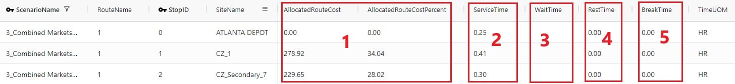
The Transportation Stop Summary output table lists for each route all the individual stops and their details around amount of product delivered, allocated cost, service time, and stop location information.
This first screenshot shows the basic details of the stops in terms of route name, stop ID, location, stop type, and how much product was delivered:
Somewhat further right on the Transportation Stop Summary table we find the outputs that detail the route cost allocation and the different types of time spent at the stop:
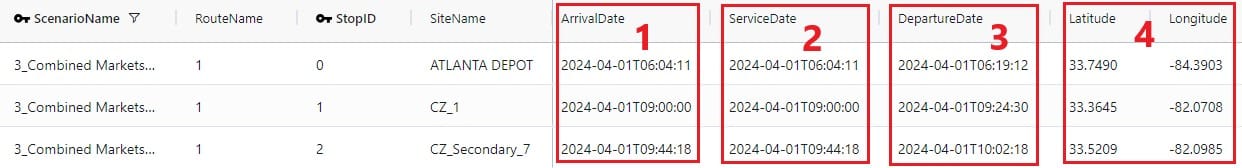
Lastly, farthest right on the Transportation Stop Summary table, arrival, service, and departure dates are listed, along with the stop’s latitude and longitude:
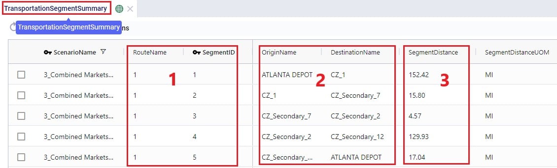
The Transportation Segment Summary output table contains distance, time, and source and destination location details for each segment (or “leg”) of each route.
The basic details of each segment are shown in the following screenshot of the Transportation Segment Summary table:
Further right on the Transportation Segment Summary output table, the time details of each segment are shown:
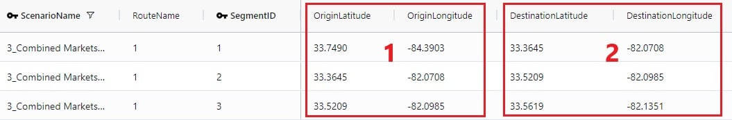
Next on the Transportation Segment Summary table are the latitudes and longitudes of the segment’s origin and destination locations:
And farthest right on the Transportation Segment Summary output table details around the start and end date and time of the segment are listed, plus CO2 emissions and the associated CO2 cost:
For each Tour (= asset schedule) the Transportation Tour Summary output table summarizes the costs, distances, times, and CO2 details.
The next 3 screenshots show the basic tour details and all costs associated with a tour:
The next screenshot shows the distance outputs available for each tour on the Transportation Tour Summary output table:
Scrolling further right on the Transportation Tour Summary table, the outputs available for tour times are listed:
If a load balancing scenario has been run (see the Load Balancing Demand input table further above for more details on how to run this), then the Transportation Load Balancing Summary output table will be populated too. Details on amount of product delivered, plus the number of routes, assets and delivered shipments by day of the week can be found in this output table; see the following 2 screenshots:
For each route, the Transportation Activity Report details all the activities that happen in chronological order with details around distance and time and it breaks down how far along the duty and drive times are at each point in the route, which is very helpful to understand when rests and short breaks are happening.
This first screenshot of the Transportation Activity Report shows the basic details of the activities:
Next, the distance, time, and delivered amount of product are detailed on the Transportation Activity Report:
Finally, the last several fields on the Transportation Activity Report details cost, and the thus far accumulated duty and drive times:
As with the other engines within Cosmic Frog, Maps are very helpful in visualizing baseline and scenario outputs. Here, we will discuss how to set up Hopper specific Maps at a high level; we will not cover all the ins and outs of maps. If you are unfamiliar with the Maps module in Cosmic Frog, then please review the “Getting Started with Maps” article in the Optilogic Help Center first. It covers how to add and configure new maps and their layers.
Visualizing Hopper routes and direct shipments on maps is achieved by adding map layers which use 1 of the following as the table name:
Using what we have discussed above and the learnings from the Getting Started with Maps help center article, we can create the following map quite easily and quickly (the model used here is one from the Resource Library, named Transportation Optimization):
The steps taken to create this map are:
Let’s also cover 2 maps of a model where both pickups and deliveries are being made, from “backhaul” and to “linehaul” customers, respectively. When setting the LIFO (Is Last In First Out) field on the Transportation Assets table to True, this leads to routes that contain both pickup and delivery stops, but all the pickups are made at the end (e.g. modeling backhaul):
Two example routes are being shown in the screenshot above and we can see that all deliveries are first made to the linehaul customers which have blue icons. Then, pickups are made at the backhaul customers which have orange icons. If we want to design interleaved routes where pickups and deliveries can be mixed, we need to set the LIFO field to False. The following screenshot shows 2 of these interleaved routes:
The above 2 screenshots use the Transportation Routes Map Layer as the table name to draw the Routes map layer, where the condition builder is used to filter for 2 of the route names.
Finally, we will go back to the Transportation Optimization model which was used for the first map screenshot in this section. The Baseline scenario in this model has 1 shipment that is being shipped directly. To visualize this on the map we add a map layer named "Direct Shipping" which uses the Transportation Shipment Summary as the table name input. On the Layer Style pane we change the color for this line layer to red. We also keep the "Routes" map layer, which is drawn from the Transportation Routes Map Layer with the default dark blue color:
In the Analytics module of Cosmic Frog, dashboards that show graphs of scenario outputs, sliced and diced to the user’s preferences, can quickly be configured. Like Maps, this functionality is not Hopper specific and other Cosmic Frog technologies use these extensively too. We will cover setting up a Hopper specific visualization, but not all the details of configuring dashboards. Please review these resources on Analytics in Cosmic Frog first if you are not yet familiar with these:
We will do a quick step by step walk through of how to set up a visualization of comparing scenario costs by cost type in a new dashboard:
The steps to set this up are detailed here, note that the first 4 bullet points are not shown in the screenshot above:
There are several models in the Resource Library that transportation optimization users may find helpful to review. How to use resources in the Resource Library is described in the help center article “How to Use the Resource Library”.