Depending on the type of supply chain one is modelling in Cosmic Frog and the questions being asked of it, it may be necessary to utilize some or all the features that enable detailed production modelling. A few business case examples that will often include some level of detailed production modelling include:
In comparison, modelling a retailer who buys all its products from suppliers as finished goods, does not require any production details to be added to its Cosmic Frog model. Hybrid models are also possible, think for example of a supermarket chain which manufactures its own branded products and buys other brands from its suppliers. Depending on the modelling scope, the production of the own branded products may require using some of the detailed production features.
The following diagram shows a generalized example of production related activities at a manufacturing plant, all of which can be modelled in Cosmic Frog:

In this help article we will cover the inputs & outputs of Cosmic Frog’s production modelling features, while also giving some examples of how to model certain business questions. The model in Optilogic’s Resource Library that is used mainly for the screenshots in this article is the Multi-Year Capacity Planning. There is a 20-minute video available with this model in the Resource Library, which covers the business case that is modelled and some detail of the production setup too.
To not make this document too repetitive we will cover some general Cosmic Frog functionality here that applies to all Cosmic Frog technologies and is used extensively for production modelling in Neo too.
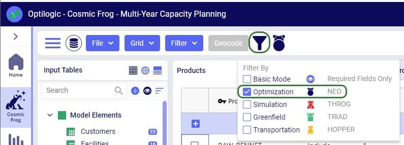
To only show tables and fields in them that can be used by the Neo network optimization algorithm, select Optimization in the Technologies Filter from the toolbar at the top in Cosmic Frog. This will hide any tables and fields that are not used by Neo and therefore simplifies the user interface.
Quite a few Neo related fields in the input and output tables will be discussed in this document. Keep in mind however that a lot of this information can also be found in the tooltips that are shown when you hover over the column name in a table, see following screenshot for an example. The column name, technology/technologies that use this field, a description of how this field is used by those algorithm(s), its default value, and whether it is part of the table’s primary key are listed in the tooltip.
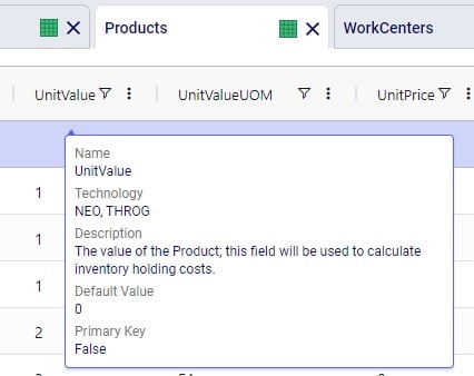
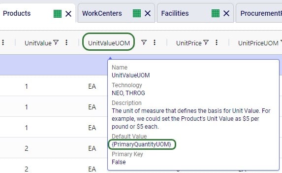
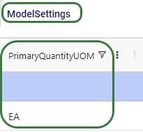
There are a lot of fields with names that end in “…UOM” throughout the input tables. How they work will be explained here so that individual UOM fields across the tables do not need to be explained further in this documentation as they all work similarly. These UOM fields are unit of measure fields and often appear to the immediate right of the field that they apply to, like for example Unit Value and Unit Value UOM in the screenshot above. In these UOM fields you can type the Symbol of a unit of measure that is of the required Type from the ones specified in the Units Of Measure input table. For example, in the screenshot above, the unit of measure Type for the Unit Value UOM field is Quantity. Looking in the Units Of Measure input table, we see there are 2 of these specified: Each and Pallet, with Symbol = EA and PLT, respectively. We can use either of these in this UOM field. If we leave a UOM field blank, then the Primary UOM for that UOM Type specified in the Model Settings input table will be used. For example, for the Unit Value UOM field in the screenshot above the tooltip says Default Value = {Primary Quantity UOM}. Looking this up in the Model Settings table shows us that this is set to EA (= each) in our current model. Let’s illustrate this with the following screenshots of 1) the tooltip for the Unit Value UOM field (located on the Products input table), 2) units of measure of Type = Quantity in the Units Of Measure input table and 3) checking what the Primary Quantity UOM is set to in the Model Settings input table, respectively:

Note that only hours (Symbol = HR) is currently allowed as the Primary Time UOM in the Model Settings table. This means that if another Time UOM, like for example minutes (MIN) or days (DAY), is to be used, the individual UOM fields need to be utilized to set these. Leaving these blank would mean HR is used by default.
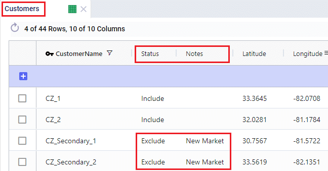
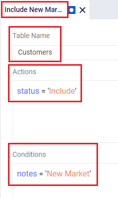
With few exceptions, all tables in Cosmic Frog contain both a Status field and a Notes field. These are often used extensively to add elements to a model that are not currently part of the supply chain (commonly referred to as the “Baseline”), but are to be included in scenarios in case they will definitely become part of the future supply chain or to see whether there are benefits to optionally include these going forward. In these cases, the Status in the input table is set to Exclude and the Notes field often contains a description along the lines of ‘New Market’, ‘New Line 2026’, ‘Alternative Recipe Scenario 3, ‘Faster Bottling Plant5 China’, ‘Include S6’, etc. When creating scenario items for setting up scenarios, the table can then be filtered for Notes = ‘New Market’ while setting Status = ‘Include’ for those filtered records. We will not call out these Status and Notes fields in each individual input table in the remainder of this document, but we do encourage users to use these extensively as they make creating scenarios very easy. When exploring any Cosmic Frog models in the Resource Library, you will notice the extensive use of these fields too. The following 2 screenshots illustrate the use of the Status and Notes fields for scenario creation: 1) shows several customers on the Customers table where CZ_Secondary_1 and CZ_Secondary_2 are not currently customers that are being served but we want to explore what it takes to serve them in future. Their Status is set to Exclude and the Notes field contains ‘New Market’; 2) a scenario item called ‘Include New Market’ shows that the Status of Customers where Notes = ‘New Market’ is changed to ‘Include’.
The Status and Notes fields are also often used for the opposite where existing elements of the current supply chain are excluded in scenarios in cases where for example manufacturing locations, products or lines are going to go offline in the future. To learn more about scenario creation, please see this short Scenarios Overview video, this Scenario Creation and Maps and Analytics training session video, this Creating Scenarios in Cosmic Frog help article, and this Writing Scenario Syntax help article.
The model that is mostly used for screenshots throughout this help article is as mentioned above the Multi-Year Capacity Planning model that can be found here in the Resource Library. This model represents a European cheese supply chain which is used to make investment decisions around the growth of a non-mature market in Eastern Europe over a 5-year modelling horizon. New candidate DCs are considered to serve the growing demand in Eastern Europe, the model optimizes which are optimal to open and during which of the 5 years of the modelling horizon. The production setup in the model uses quite a few of the detailed modelling features which will be discussed in detail in this document:
Note that in the screenshots of this model, the columns have been re-ordered sometimes, so you may see a different order in your Cosmic Frog UI when opening the same tables of this model.
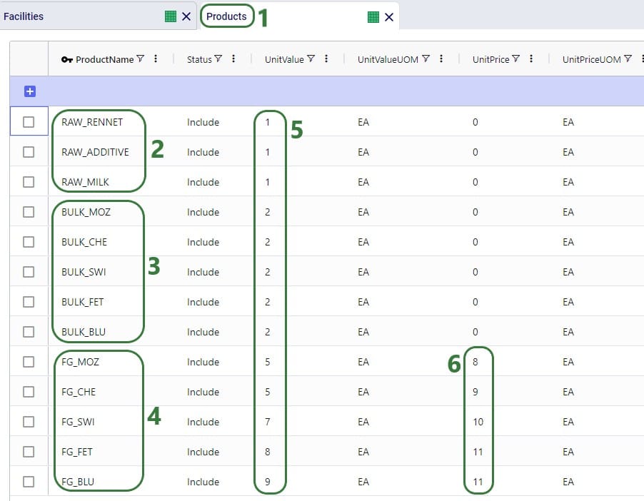
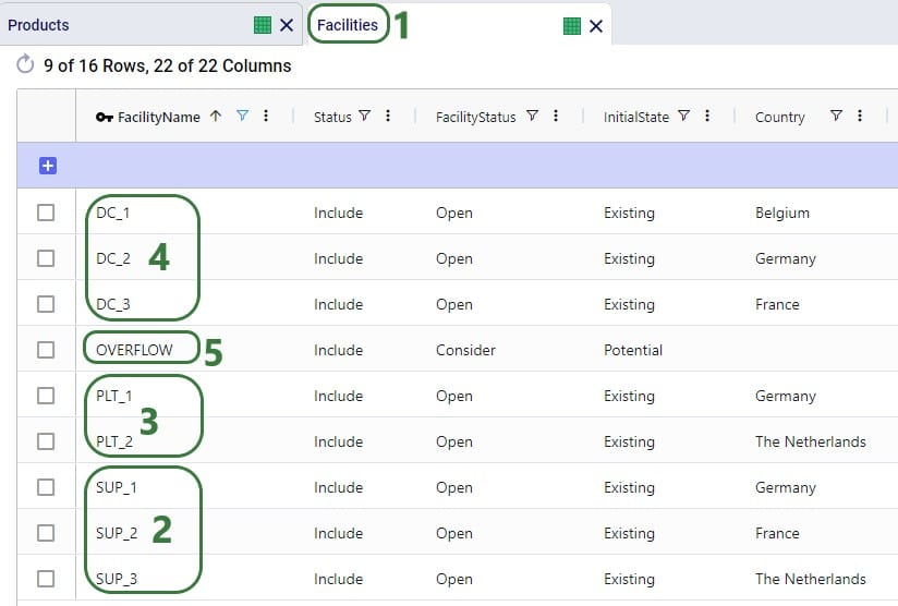
The 2 screenshots below show the Products and Facilities input tables of this model in Cosmic Frog:
Note that the naming convention of the products lends itself to easy filtering of the table for the raw materials, bulk materials, and finished goods due to the RAW_, BULK_, and FG_ prefixes. This makes the creation of groups and setting up of scenarios quick and easy.
Note that similar to the naming convention of the products, the facilities are also named with prefixes that facilitate filtering of the facilities so groups and scenarios can quickly be created.
Here is a visual representation of the model with all facilities and customers on the map:

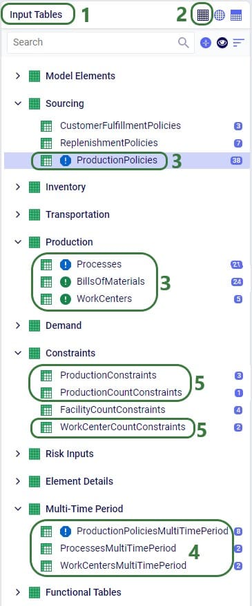
The specific features in Cosmic Frog that allow users to model and optimize production processes of varying levels of complexity while using the network optimization engine (Neo) include the following input tables:
We will cover all these production related input tables to some extent in this article, starting with a short description of each of the basic single-period input tables:
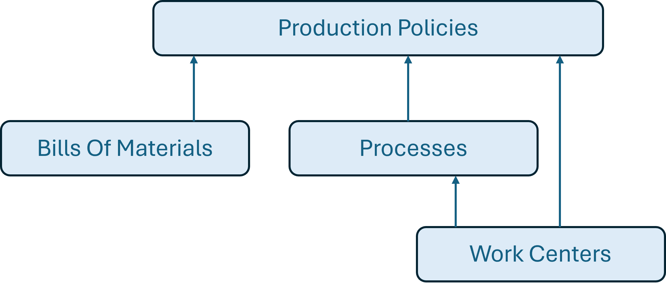
These 4 tables feed into each other as follows:
A couple of notes on how these tables work together:
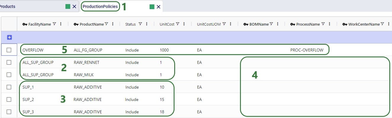
For all products that are explicitly modelled in a Cosmic Frog model, there needs to be at least 1 policy specified on the Production Policies table or the Supplier Capabilities table so there is at least 1 origin location for each. This applies to for example raw materials, intermediates, bulk materials, and finished goods. The only exception is if by-products are being modelled, these can have Production Policies associated with them, but do not necessarily need to (more on this when discussing Bills of Materials further below). From the 2 screenshots below of the Production Policies table, it becomes clear that depending on the type of product and the level of detail that is needed for the production elements of the supply chain, production policies can be set up quite differently: some use only a few of the fields, while others use more/different fields.
A couple of notes as follows:
Next, we will look at a few other records on the Production Policies input table:

We will take a closer look at the BOMs and Processes specified on these records when discussing the Bills of Materials and Processes tables further below.
Note that the above screenshot was just for PLT_1 and mozzarella, there are similar records in this model for the other 4 cheeses which can also be made at PLT_1, plus similar records for all 5 cheeses at PLT_2, which includes a new potential production line for future expansion too.
Other fields on the Production Policies table that are not shown in the above 2 screenshots are:
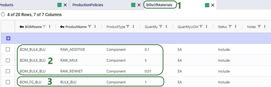
The recipes of how materials/products of different stages convert into each other are specified on the Bills of Materials (BOMs) table. Here the BOMs for the blue cheese (_BLU) products are shown:
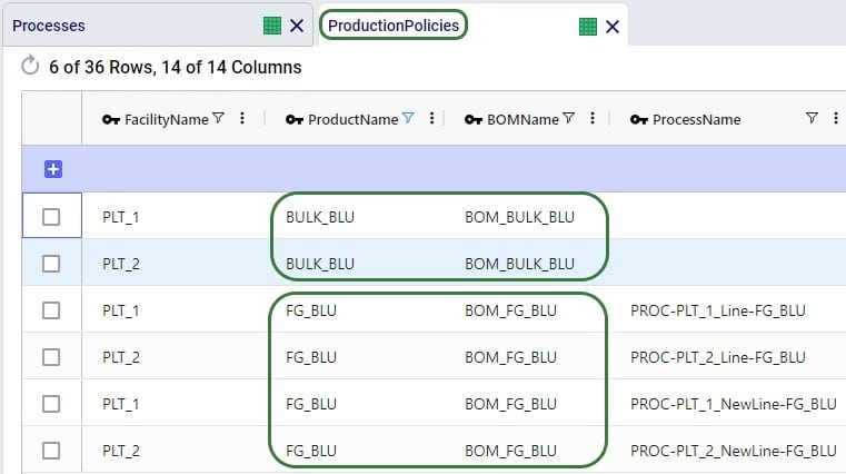
Note that the above specified BOMs are both location and end-product agnostic. Their names suggest that they are specific for making the BULK_BLU and FG_BLU products, but only associating these BOMs on a Production Policy which has Product Name set to these makes this connection. We can use these BOMs at any location that they apply. Filtering the Production Policies table for the BULK_BLU and FG_BLU products we can see that 1) BOM_BULK_BLU is indeed used to make BULK_BLU and BOM_FG_BLU to make FG_BLU, and 2) the same BOMs are used at PLT_1 and PLT_2:
It is of course possible that the same product uses a different BOM at a different location. In this case, users can set up multiple BOMs for this product on the BOMs table and associate the correct one at the correct location in the Production Policies table. Choosing a naming convention for the BOM Names that includes the location name (or a code to indicate it) is recommended.
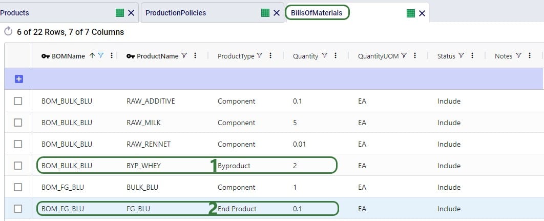
The screenshot above of the Bills of Materials table only shows records with Product Type = Component. Components are input into a BOM and are consumed by it when producing the end-product. Besides Component, Product Type can also be set to End Product or Byproduct. We will explain these 2 product types through the examples in this following screenshot:
Notes:
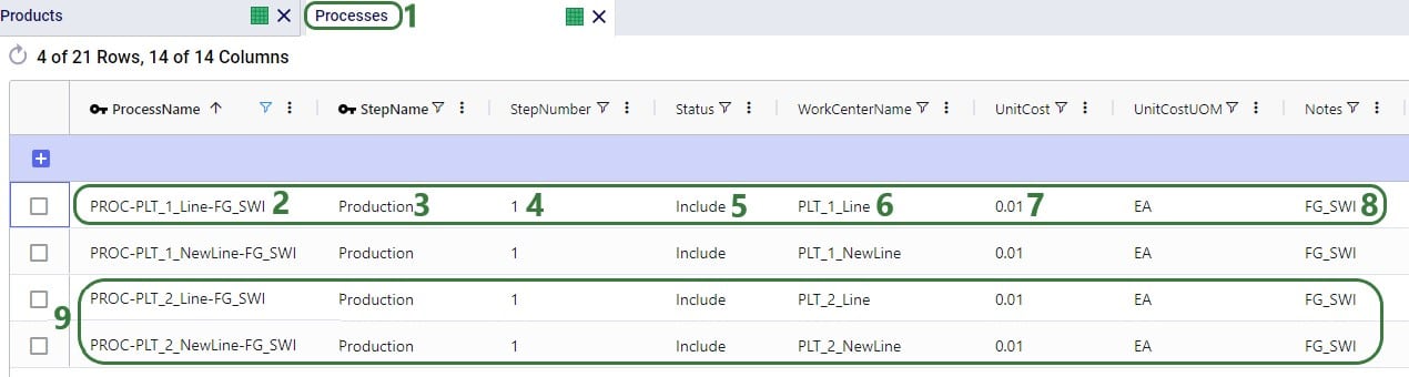
On the Processes table production processes of varying levels of complexity can be set up, from simple 1 step processes without using any work centers, to multi-step ones that specify costs, processing rates, and use different work centers for each step. The processes specified in the Multi-Year Capacity Planning model are relatively straightforward:
Let us also look at an example in a different model which contains somewhat more complex processes for a car manufacturer where the production process can roughly be divided into 3 steps:

Note that, like BOMs, Processes can in theory be both location and end-product agnostic. However:
Other fields on the Processes table that are not shown in the above 2 screenshots are:
If it is important to capture costs and/or capacities of equipment like production lines, tools, machines that are used in the production process, these can be modelled by using work centers to represent the equipment:
In the above screenshot, 2 work centers are set up at each plant: 1 existing work center and 1 new potential work center. The new work centers (PLT_1_NewLine and PLT_2_NewLine) have Work Center Status set to Closed, so they will not be considered for inclusion in the network when running the Baseline scenario. In some of the scenarios in the model, the Work Center Status of these 2 lines is changed to Consider and in these scenarios one of the new lines or both can be opened and used if it is optimal to do so. The scenario item that makes this change looks like this:
Next, we will also look at a few other fields on the Work Centers table that the Multi-Year Capacity Planning model utilizes:
In theory, it can be optimal for a model to open a considered potential work center in one period of the model (say 2024 in this model), close it again in a later period (e.g. 2025), for it then to open it again later (e.g. 2026), etc. In this case Fixed Startup or Fixed Closing Costs would be applied each time the work center was opened or closed, respectively. This type of behavior can be undesirable and is by default prevented by a Neo Run Parameter called “Open Close At Most Once”, as shown in this screenshot:

After clicking on the Run button, the Run screen comes up. The “Open Close At Most Once” parameter can be found in the Neo (Optimization) Parameters section. By default, it is turned on, meaning that a work center or facility is only allowed to change state once during the model’s horizon, i.e. once from closed to open if the Initial State = Potential or once from open to closed if the Initial State = Existing. There may however be situations where opening and/or closing of work centers and facilities multiple times during the model horizon is allowable. In that case, the Open Close At Most Once parameter can be turned off.
Other fields on the Work Centers table that are not shown in the above screenshots are:
Fixed Operating, Fixed Startup, and Fixed Closing Costs can be stepped costs. These can be entered into the fields on the Work Centers input table directly or can be specified on the Step Costs input table and then used on the Work Centers table in those cost fields. An example of stepped costs set up in the Step Costs input table is shown in the screenshot below where the costs are set up to capture the weekly shift cost for 1 person (note that these stepped costs are not in the Multi-Year Capacity Planning model in the Resource Library, they are shown here as an additional example):
To set for example the Fixed Operating Cost to use this stepped cost, type “WC_Shifts” into the Fixed Operating Cost field on the Work Centers input table.
Many of the input tables in Cosmic Frog have a Multi-Time Period equivalent, which can be used in models that have more than 1 period. These tables enable users to make changes that only apply to specific periods of the model. For example, to:
The multi-time period tables are copies of their single-period equivalents, with a few columns added and removed (we will see examples of these in screenshots further below):
Notes on switching status of records through the multi-period tables and updating records partially:
Three of the 4 production specific input tables that have been discussed above have a multi-time period equivalent: Production Policies, Processes, and Work Centers. There is no equivalent for the Bills Of Materials input table, as BOMs are only used if they are associated on records in the Production Policies table. Using different BOMs during different periods can be achieved by associating those BOMs on the Production Policies single-period table and setting the Status of them to Include for those to be used for most of the periods and to Exclude if they are to be included for certain periods / scenarios. Then add those records for which the Status needs to be switched to the Production Policies multi-period input table (we will walk through an example of this using screenshots in the next section).
The 3 production specific multi-time period input tables do have all of the same fields as their single-period equivalents, with the addition of the Period Name field and additional Status field. We will not discuss each multi-time period table and all its fields in detail here, but rather give a few examples of how each can be used.
Note that from this point onwards the Multi-Year Capacity Planning model was modified and added to for purposes of this help article, the version in the Resource Library does not contain the same data in the Multi-Time Period input tables and production specific Constraint tables that is shown in the screenshots below.
This first example on the Production Policies Multi-Time Period input table shows how the production of the cheddar finished good (FG_CHE) is prevented at plant 1 (PLT_1) in years 4 and 5 of the model:
In the following example, an alternative BOM to make feta (FG_FET) is added and set to be used at Plant 2 (PLT_2) during all periods instead of the original BOM. This is set up to be used in a scenario, so the original records need to be kept intact for the Baseline and other scenarios. To set this up, we need to update the Bills Of Materials, Production Policies, and Production Policies Multi-Time Period table, see the following screenshots and explanations:

On the Bills Of Materials input table, all we need to do is add the records for the new BOM that results in FG_FET. It has 2 records, both named ALTBOM_FG_FET, and instead of using only BULK_FET as the component which is what the original BOM uses, it uses a mix of BULK_FET and BULK_BLU as its components.
Next, we first need to associate this new BOM through the Production Policies table:
Lastly, the records that need to be added to the Production Policies Multi-Time Period table are the following 4 which have all the same values for the key columns as the 4 records in the above screenshot of the Production Policies single-period input table, which contain all the possible ways to produce FG_FET at PLT_2:
In the following example, we want to change the unit cost on 2 of the processes: at Plant 1 (PLT_1), the cost on the new potential line needs to be decreased to 0.005 for cheddar cheese (CHE) and increased to 0.015 for Swiss cheese (SWI). This can be done by using the Processes Multi-Time Period input table:
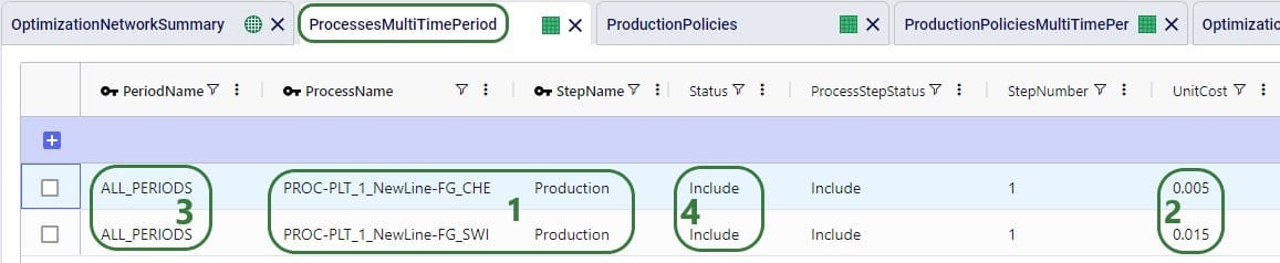
Note that there is also a Work Center Name field on the Processes Multi-Time Period table (not shown in the screenshot). As this is not a key field on the Processes input tables, it can be left blank here on the multi-time period table. This field will not be changed and the value from the single-time period table Work Center Name field will be used for these 2 records.
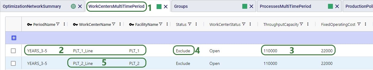
In the following example, we want to evaluate if upgrading the existing production lines at both plants from the 3rd year of the modelling horizon onwards, so they have a higher throughput capacity at a somewhat higher fixed operating cost, is a good alternative to opening one of the potential new lines at either plant. First, we add a new periods group to the model to set this up:
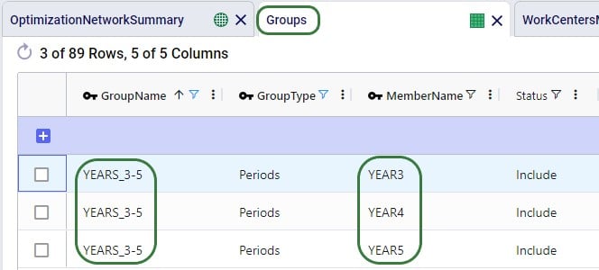
On the Groups table, we set up a new group named YEARS3-5 (Group Name) that is of Group Type = Periods and has 3 members: YEAR3, YEAR4 and YEAR5 (Member Name).
Cosmic Frog contains multiple tables through which different types of constraints can be added to network optimization (Neo) models. A constraint limits the model in a certain part of the network. These limits can for example be lower or upper limits in terms of the amount of flow between certain locations or certain echelons, the amount of inventory of a certain product or product group at a specific location or network wide, the amount of production of a certain product or product group at a specific location or network wide, etc. In this section the 3 constraints tables that are production specific will be covered: Production Constraints, Production Count Constraints, and Work Center Count Constraints.
A couple of general notes on all constraints tables:
In this example, we want to add constraints to the model that limit the production of all 5 finished goods together to 90,000 units. Both plants have this same upper production limit across the finished goods, and the limit applies to each year of the modelling horizon (5 yearly periods).

Note that there are more fields on the Production Constraints input table which are not shown in the above screenshot. These are:
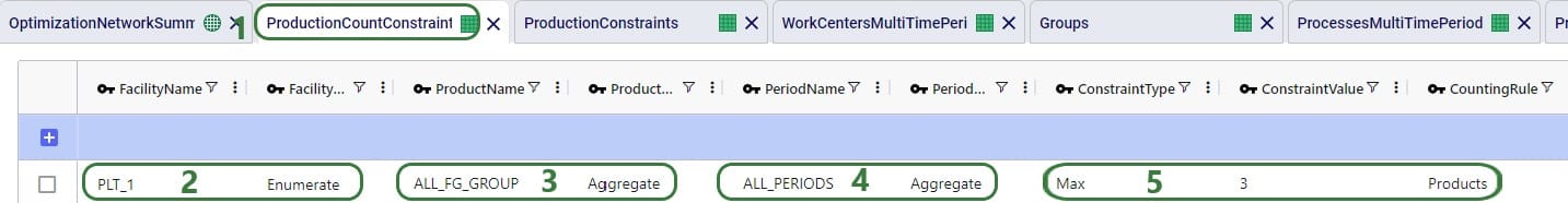
In this example, we want to limit the number of products that are produced at PLT_1 to a maximum of 3 (out of the 5 finished goods). This limit applies over the whole 5-year modelling period, meaning that in total PLT_1 can produce no more than 3 finished goods:
Again, note there are more fields on the Production Count Constraints input table which are not shown in the above screenshot. These are:
Next, we will show an example of how to open at least 3 work centers, but no more than 5 out of 8 candidate work centers. These limits apply to all 5 yearly periods in the model together and over all facilities present in the model.

Again, there are more fields on the Work Center Count Constraints table that are not shown in the above screenshot:
After running a network optimization using Cosmic Frog’s Neo technology, production specific outputs can be found in several of the more general output tables, like the Optimization Network Summary, and the Optimization Constraints Summary (if any constraints were applied). Outputs more focused on just production can be found in 4 production specific output tables: the Optimization Production Summary, the Optimization Bills Of Material Summary, the Optimization Process Summary, and the Optimization Work Center Summary. We will cover these tables here, starting with the Optimization Network Summary.
The following screenshot shows the production specific outputs that are contained in the Optimization Network Summary output table:
Other production related fields on this table which are not shown in the screenshot above are:
The Optimization Production Summary output table has a record with the production details for each product that was produced as part of the model run:
Other fields on this output table which are not shown in the screenshot are:
The details of how many components were used and how much by-product produced as a result of any bills of materials that were used as part of the production process can be found on the Optimization Bills Of Material Summary output table:
Note that aside from possibly knowing based on the BOM Name, it is not listed in the Bills Of Material Summary output table what the end product is and how much of it is produced as a result of a BOM. Those details are contained in the Optimization Production Summary output table discussed above.
Other fields on this output table which are not shown in the screenshot are:
The details of all the steps of any processes used as part of the production in the Neo network optimization run can be found in the Optimization Process Summary, see these next 2 screenshots:

Other fields on this output table which are not shown in the screenshots are:
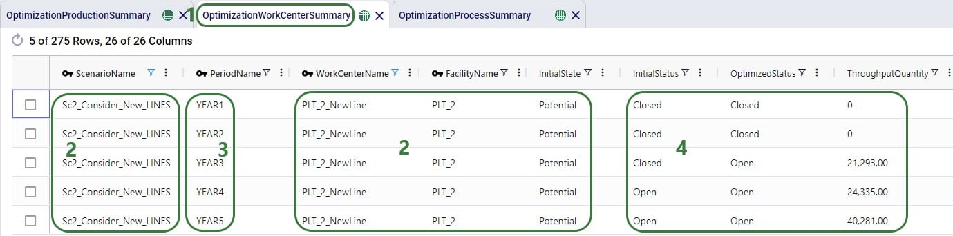
For each Work Center that has its Status set to Include or Consider, a record for each period of the model can be found in the Optimization Work Center Summary output table. It summarizes if the Work Center was used during that period, and, if so, how much and at what cost:
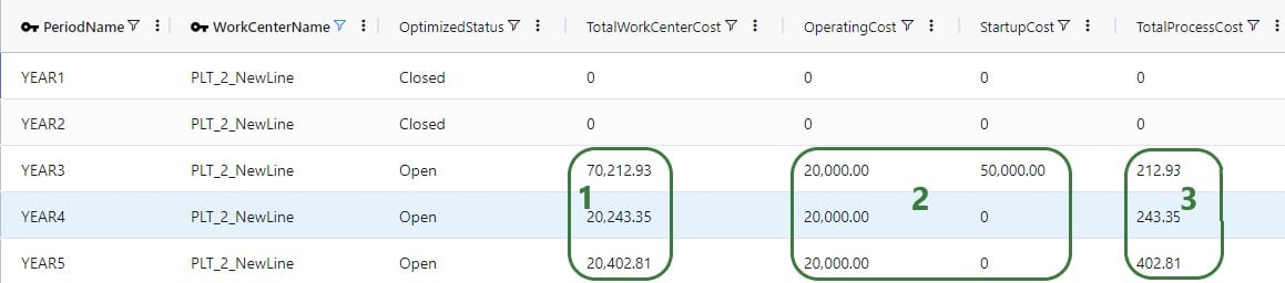
The following screenshot shows a few more output fields on the Optimization Work Center Summary output tables that have non-0 values in this model:
Other fields on this output table which are not shown in the screenshots are:
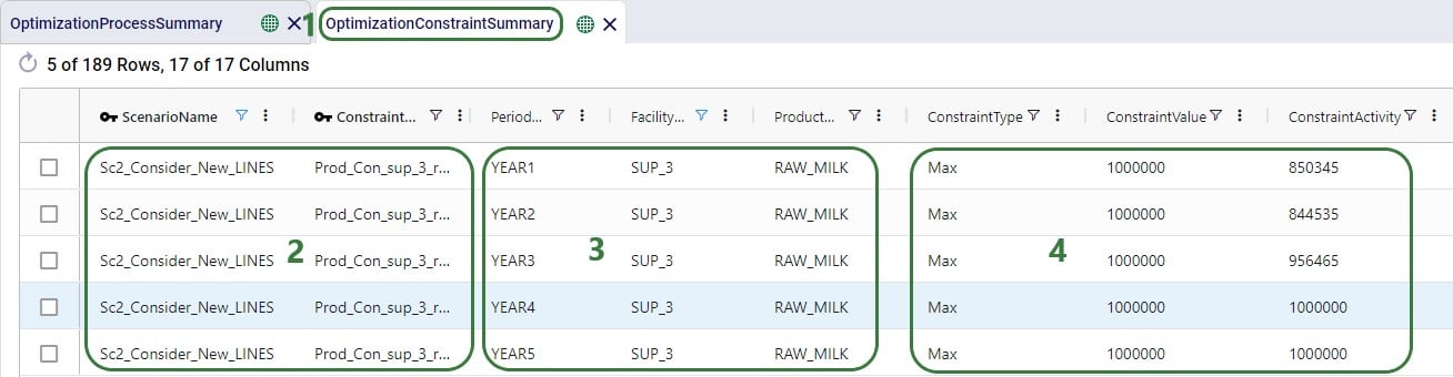
For all constraints in the model, the Optimization Constraint Summary can be a very handy table to check if any constraints are close to their maximum (or minimum, etc.) value to understand where the current and future bottlenecks are and likely will be. The screenshot below shows the outputs on this table for a production constraint that is applied at each of the 3 suppliers, where neither can produce more than 1 million units of RAW_MILK in any 1 year. In the screenshot we specifically look at the Supplier named SUP_3:
Other fields on this output table which are not shown in the screenshots are:
There are a few other output tables of which the main outputs are not related to production, but still contain several fields that result from productions. These are:
In this help article we have covered how to set up alternative Work Centers at existing locations and use the Work Center Status and Initial State fields to evaluate if including these, and from what period onwards if so, will be optimal. We have also covered how Work Center Count Constraints can be used to pick a certain amount of Work Centers to be opened/used from a set of multiple candidates, either at 1 location or multiple. Here we also want to mention that Facility Count Constraints can be used when making decisions at the plant level. Say that based on market growth in a certain region, a manufacturer decides a new plant needs to be built. There are 3 candidate locations for the plant from which the optimal needs to be picked. This can be set up as follows in Cosmic Frog:
A couple of alternative approaches to this are:
As mentioned above in the section on the Bill Of Materials input table, it is possible to set up a model where there is demand for a product that is the By-product resulting from a BOM. This does require some additional set up, and the below walks through this, while also showcasing how the model can be used to determine how much of any flexible demand for this by-product to fulfill. The screenshots show the set-up of a very simple example model built for this specific purpose.
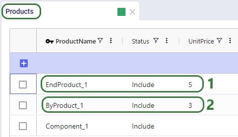
On the Products table, besides the component (for which there also is demand in this model) that goes into any BOM, we also specify:

The demand for the 3 products is set up on the Customer Demand table and we notice that 1) there is demand for the Component, the End Product, and the By-Product, and 2) the Demand Status for ByProduct_1 is set to Consider, which means it does not need to be fulfilled, it will be (partially) fulfilled if it is optimal to do so. (For Component_1 and EndProduct_1 the Demand Status field is left blank, which means the default value of Include will be used.)
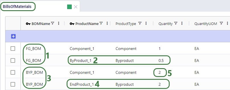
The EndProduct_1 is made through a BOM which consumes Component_1 and also make ByProduct_1 as a Byproduct. For this we need to set up a BOM:

Next, on the Production Policies table, we see that Component_1 can be created without a BOM, and:
In reality, these 2 production policies result in the same consumption of Component_1 and same production amounts of EndProduct_1 and ByProduct_1. Both need to be present however in order to be able to also have demand for ByProduct_1 in the model.
Other model elements that need to be set up are:
Three scenarios were run for this simple example model with the only difference between them the Unit Price for ByProduct_1: Baseline (price of ByProduct_1 = 3), PriceByproduct1 (Unit Price of ByProduct_1 = 1), PriceByproduct2 (Unit Price of ByProduct_1 = 2). Let’s review some of the outputs to understand how this Unit Price affects the fulfillment of the flexible demand for ByProduct_1:
The high-level costs, revenues, profit and served/unserved demand outputs by scenario can be found on the Optimization Network Summary output table:
On the Optimization Production Summary output table, we see that all 3 scenarios used BYP_BOM for the production of EndProduct_1 and ByProduct_1, it could have also picked the other BOM (FG_BOM) and the overall results would have been the same.
As the Optimization Production Summary only shows the production of the end products, we will also have a look at the Optimization Bills Of Material Summary output table:
Lastly, we will have a look at the Optimization Inventory Summary output table:
Note that had the demand for Byproduct_1 been set to Include rather than Consider in this example model, all 3 scenarios would have produced 100 units of it to fulfill the demand, and as a result have produced 200 units of EndProduct_1. 100 of those would have been used to fulfill the demand for EndProduct_1 and the other 100 would have stayed in inventory, like we saw in the Baseline scenario above.
Depending on the type of supply chain one is modelling in Cosmic Frog and the questions being asked of it, it may be necessary to utilize some or all the features that enable detailed production modelling. A few business case examples that will often include some level of detailed production modelling include:
In comparison, modelling a retailer who buys all its products from suppliers as finished goods, does not require any production details to be added to its Cosmic Frog model. Hybrid models are also possible, think for example of a supermarket chain which manufactures its own branded products and buys other brands from its suppliers. Depending on the modelling scope, the production of the own branded products may require using some of the detailed production features.
The following diagram shows a generalized example of production related activities at a manufacturing plant, all of which can be modelled in Cosmic Frog:
In this help article we will cover the inputs & outputs of Cosmic Frog’s production modelling features, while also giving some examples of how to model certain business questions. The model in Optilogic’s Resource Library that is used mainly for the screenshots in this article is the Multi-Year Capacity Planning. There is a 20-minute video available with this model in the Resource Library, which covers the business case that is modelled and some detail of the production setup too.
To not make this document too repetitive we will cover some general Cosmic Frog functionality here that applies to all Cosmic Frog technologies and is used extensively for production modelling in Neo too.
To only show tables and fields in them that can be used by the Neo network optimization algorithm, select Optimization in the Technologies Filter from the toolbar at the top in Cosmic Frog. This will hide any tables and fields that are not used by Neo and therefore simplifies the user interface.
Quite a few Neo related fields in the input and output tables will be discussed in this document. Keep in mind however that a lot of this information can also be found in the tooltips that are shown when you hover over the column name in a table, see following screenshot for an example. The column name, technology/technologies that use this field, a description of how this field is used by those algorithm(s), its default value, and whether it is part of the table’s primary key are listed in the tooltip.
There are a lot of fields with names that end in “…UOM” throughout the input tables. How they work will be explained here so that individual UOM fields across the tables do not need to be explained further in this documentation as they all work similarly. These UOM fields are unit of measure fields and often appear to the immediate right of the field that they apply to, like for example Unit Value and Unit Value UOM in the screenshot above. In these UOM fields you can type the Symbol of a unit of measure that is of the required Type from the ones specified in the Units Of Measure input table. For example, in the screenshot above, the unit of measure Type for the Unit Value UOM field is Quantity. Looking in the Units Of Measure input table, we see there are 2 of these specified: Each and Pallet, with Symbol = EA and PLT, respectively. We can use either of these in this UOM field. If we leave a UOM field blank, then the Primary UOM for that UOM Type specified in the Model Settings input table will be used. For example, for the Unit Value UOM field in the screenshot above the tooltip says Default Value = {Primary Quantity UOM}. Looking this up in the Model Settings table shows us that this is set to EA (= each) in our current model. Let’s illustrate this with the following screenshots of 1) the tooltip for the Unit Value UOM field (located on the Products input table), 2) units of measure of Type = Quantity in the Units Of Measure input table and 3) checking what the Primary Quantity UOM is set to in the Model Settings input table, respectively:
Note that only hours (Symbol = HR) is currently allowed as the Primary Time UOM in the Model Settings table. This means that if another Time UOM, like for example minutes (MIN) or days (DAY), is to be used, the individual UOM fields need to be utilized to set these. Leaving these blank would mean HR is used by default.
With few exceptions, all tables in Cosmic Frog contain both a Status field and a Notes field. These are often used extensively to add elements to a model that are not currently part of the supply chain (commonly referred to as the “Baseline”), but are to be included in scenarios in case they will definitely become part of the future supply chain or to see whether there are benefits to optionally include these going forward. In these cases, the Status in the input table is set to Exclude and the Notes field often contains a description along the lines of ‘New Market’, ‘New Line 2026’, ‘Alternative Recipe Scenario 3, ‘Faster Bottling Plant5 China’, ‘Include S6’, etc. When creating scenario items for setting up scenarios, the table can then be filtered for Notes = ‘New Market’ while setting Status = ‘Include’ for those filtered records. We will not call out these Status and Notes fields in each individual input table in the remainder of this document, but we do encourage users to use these extensively as they make creating scenarios very easy. When exploring any Cosmic Frog models in the Resource Library, you will notice the extensive use of these fields too. The following 2 screenshots illustrate the use of the Status and Notes fields for scenario creation: 1) shows several customers on the Customers table where CZ_Secondary_1 and CZ_Secondary_2 are not currently customers that are being served but we want to explore what it takes to serve them in future. Their Status is set to Exclude and the Notes field contains ‘New Market’; 2) a scenario item called ‘Include New Market’ shows that the Status of Customers where Notes = ‘New Market’ is changed to ‘Include’.
The Status and Notes fields are also often used for the opposite where existing elements of the current supply chain are excluded in scenarios in cases where for example manufacturing locations, products or lines are going to go offline in the future. To learn more about scenario creation, please see this short Scenarios Overview video, this Scenario Creation and Maps and Analytics training session video, this Creating Scenarios in Cosmic Frog help article, and this Writing Scenario Syntax help article.
The model that is mostly used for screenshots throughout this help article is as mentioned above the Multi-Year Capacity Planning model that can be found here in the Resource Library. This model represents a European cheese supply chain which is used to make investment decisions around the growth of a non-mature market in Eastern Europe over a 5-year modelling horizon. New candidate DCs are considered to serve the growing demand in Eastern Europe, the model optimizes which are optimal to open and during which of the 5 years of the modelling horizon. The production setup in the model uses quite a few of the detailed modelling features which will be discussed in detail in this document:
Note that in the screenshots of this model, the columns have been re-ordered sometimes, so you may see a different order in your Cosmic Frog UI when opening the same tables of this model.
The 2 screenshots below show the Products and Facilities input tables of this model in Cosmic Frog:
Note that the naming convention of the products lends itself to easy filtering of the table for the raw materials, bulk materials, and finished goods due to the RAW_, BULK_, and FG_ prefixes. This makes the creation of groups and setting up of scenarios quick and easy.
Note that similar to the naming convention of the products, the facilities are also named with prefixes that facilitate filtering of the facilities so groups and scenarios can quickly be created.
Here is a visual representation of the model with all facilities and customers on the map:
The specific features in Cosmic Frog that allow users to model and optimize production processes of varying levels of complexity while using the network optimization engine (Neo) include the following input tables:
We will cover all these production related input tables to some extent in this article, starting with a short description of each of the basic single-period input tables:
These 4 tables feed into each other as follows:
A couple of notes on how these tables work together:
For all products that are explicitly modelled in a Cosmic Frog model, there needs to be at least 1 policy specified on the Production Policies table or the Supplier Capabilities table so there is at least 1 origin location for each. This applies to for example raw materials, intermediates, bulk materials, and finished goods. The only exception is if by-products are being modelled, these can have Production Policies associated with them, but do not necessarily need to (more on this when discussing Bills of Materials further below). From the 2 screenshots below of the Production Policies table, it becomes clear that depending on the type of product and the level of detail that is needed for the production elements of the supply chain, production policies can be set up quite differently: some use only a few of the fields, while others use more/different fields.
A couple of notes as follows:
Next, we will look at a few other records on the Production Policies input table:
We will take a closer look at the BOMs and Processes specified on these records when discussing the Bills of Materials and Processes tables further below.
Note that the above screenshot was just for PLT_1 and mozzarella, there are similar records in this model for the other 4 cheeses which can also be made at PLT_1, plus similar records for all 5 cheeses at PLT_2, which includes a new potential production line for future expansion too.
Other fields on the Production Policies table that are not shown in the above 2 screenshots are:
The recipes of how materials/products of different stages convert into each other are specified on the Bills of Materials (BOMs) table. Here the BOMs for the blue cheese (_BLU) products are shown:
Note that the above specified BOMs are both location and end-product agnostic. Their names suggest that they are specific for making the BULK_BLU and FG_BLU products, but only associating these BOMs on a Production Policy which has Product Name set to these makes this connection. We can use these BOMs at any location that they apply. Filtering the Production Policies table for the BULK_BLU and FG_BLU products we can see that 1) BOM_BULK_BLU is indeed used to make BULK_BLU and BOM_FG_BLU to make FG_BLU, and 2) the same BOMs are used at PLT_1 and PLT_2:
It is of course possible that the same product uses a different BOM at a different location. In this case, users can set up multiple BOMs for this product on the BOMs table and associate the correct one at the correct location in the Production Policies table. Choosing a naming convention for the BOM Names that includes the location name (or a code to indicate it) is recommended.
The screenshot above of the Bills of Materials table only shows records with Product Type = Component. Components are input into a BOM and are consumed by it when producing the end-product. Besides Component, Product Type can also be set to End Product or Byproduct. We will explain these 2 product types through the examples in this following screenshot:
Notes:
On the Processes table production processes of varying levels of complexity can be set up, from simple 1 step processes without using any work centers, to multi-step ones that specify costs, processing rates, and use different work centers for each step. The processes specified in the Multi-Year Capacity Planning model are relatively straightforward:
Let us also look at an example in a different model which contains somewhat more complex processes for a car manufacturer where the production process can roughly be divided into 3 steps:
Note that, like BOMs, Processes can in theory be both location and end-product agnostic. However:
Other fields on the Processes table that are not shown in the above 2 screenshots are:
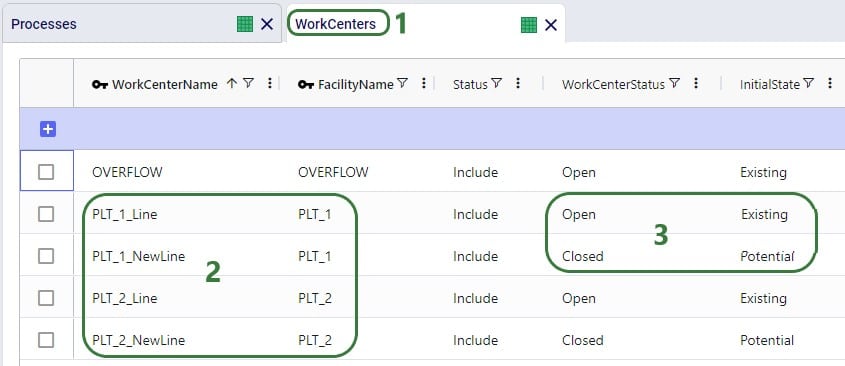
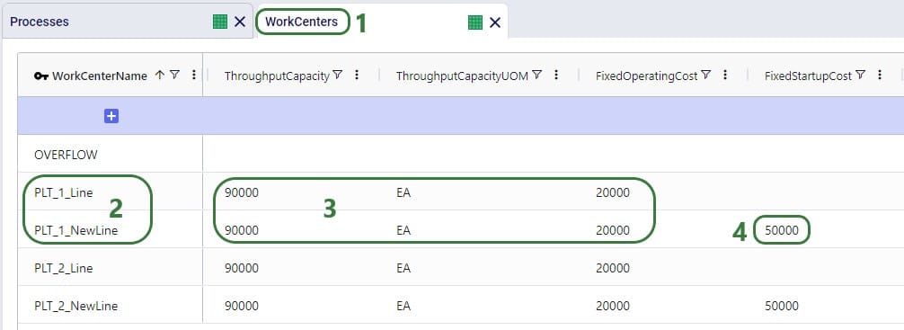
If it is important to capture costs and/or capacities of equipment like production lines, tools, machines that are used in the production process, these can be modelled by using work centers to represent the equipment:
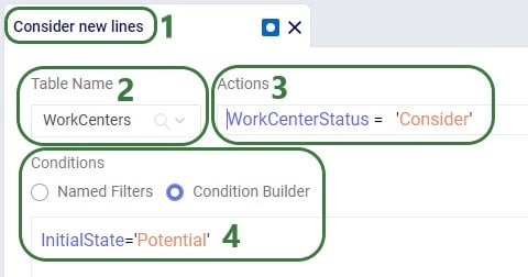
In the above screenshot, 2 work centers are set up at each plant: 1 existing work center and 1 new potential work center. The new work centers (PLT_1_NewLine and PLT_2_NewLine) have Work Center Status set to Closed, so they will not be considered for inclusion in the network when running the Baseline scenario. In some of the scenarios in the model, the Work Center Status of these 2 lines is changed to Consider and in these scenarios one of the new lines or both can be opened and used if it is optimal to do so. The scenario item that makes this change looks like this:
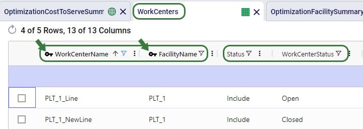
Next, we will also look at a few other fields on the Work Centers table that the Multi-Year Capacity Planning model utilizes:
In theory, it can be optimal for a model to open a considered potential work center in one period of the model (say 2024 in this model), close it again in a later period (e.g. 2025), for it then to open it again later (e.g. 2026), etc. In this case Fixed Startup or Fixed Closing Costs would be applied each time the work center was opened or closed, respectively. This type of behavior can be undesirable and is by default prevented by a Neo Run Parameter called “Open Close At Most Once”, as shown in this screenshot:
After clicking on the Run button, the Run screen comes up. The “Open Close At Most Once” parameter can be found in the Neo (Optimization) Parameters section. By default, it is turned on, meaning that a work center or facility is only allowed to change state once during the model’s horizon, i.e. once from closed to open if the Initial State = Potential or once from open to closed if the Initial State = Existing. There may however be situations where opening and/or closing of work centers and facilities multiple times during the model horizon is allowable. In that case, the Open Close At Most Once parameter can be turned off.
Other fields on the Work Centers table that are not shown in the above screenshots are:
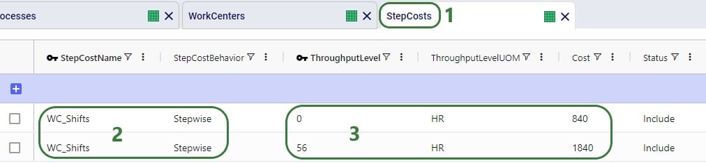
Fixed Operating, Fixed Startup, and Fixed Closing Costs can be stepped costs. These can be entered into the fields on the Work Centers input table directly or can be specified on the Step Costs input table and then used on the Work Centers table in those cost fields. An example of stepped costs set up in the Step Costs input table is shown in the screenshot below where the costs are set up to capture the weekly shift cost for 1 person (note that these stepped costs are not in the Multi-Year Capacity Planning model in the Resource Library, they are shown here as an additional example):
To set for example the Fixed Operating Cost to use this stepped cost, type “WC_Shifts” into the Fixed Operating Cost field on the Work Centers input table.
Many of the input tables in Cosmic Frog have a Multi-Time Period equivalent, which can be used in models that have more than 1 period. These tables enable users to make changes that only apply to specific periods of the model. For example, to:
The multi-time period tables are copies of their single-period equivalents, with a few columns added and removed (we will see examples of these in screenshots further below):
Notes on switching status of records through the multi-period tables and updating records partially:
Three of the 4 production specific input tables that have been discussed above have a multi-time period equivalent: Production Policies, Processes, and Work Centers. There is no equivalent for the Bills Of Materials input table, as BOMs are only used if they are associated on records in the Production Policies table. Using different BOMs during different periods can be achieved by associating those BOMs on the Production Policies single-period table and setting the Status of them to Include for those to be used for most of the periods and to Exclude if they are to be included for certain periods / scenarios. Then add those records for which the Status needs to be switched to the Production Policies multi-period input table (we will walk through an example of this using screenshots in the next section).
The 3 production specific multi-time period input tables do have all of the same fields as their single-period equivalents, with the addition of the Period Name field and additional Status field. We will not discuss each multi-time period table and all its fields in detail here, but rather give a few examples of how each can be used.
Note that from this point onwards the Multi-Year Capacity Planning model was modified and added to for purposes of this help article, the version in the Resource Library does not contain the same data in the Multi-Time Period input tables and production specific Constraint tables that is shown in the screenshots below.
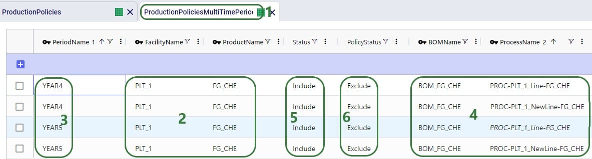
This first example on the Production Policies Multi-Time Period input table shows how the production of the cheddar finished good (FG_CHE) is prevented at plant 1 (PLT_1) in years 4 and 5 of the model:
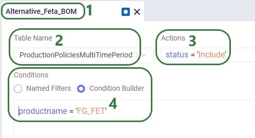
In the following example, an alternative BOM to make feta (FG_FET) is added and set to be used at Plant 2 (PLT_2) during all periods instead of the original BOM. This is set up to be used in a scenario, so the original records need to be kept intact for the Baseline and other scenarios. To set this up, we need to update the Bills Of Materials, Production Policies, and Production Policies Multi-Time Period table, see the following screenshots and explanations:
On the Bills Of Materials input table, all we need to do is add the records for the new BOM that results in FG_FET. It has 2 records, both named ALTBOM_FG_FET, and instead of using only BULK_FET as the component which is what the original BOM uses, it uses a mix of BULK_FET and BULK_BLU as its components.
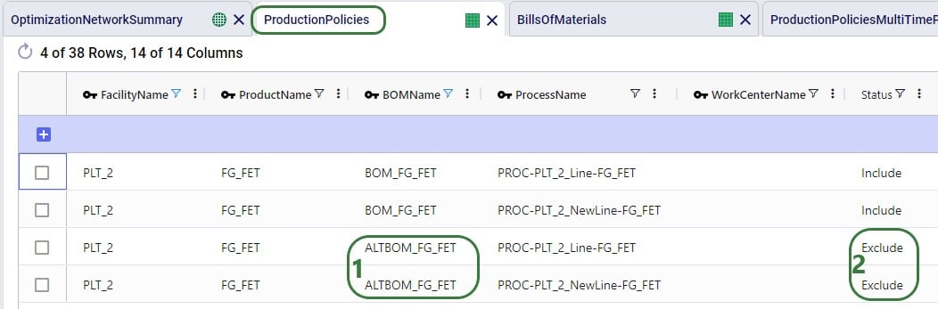
Next, we first need to associate this new BOM through the Production Policies table:
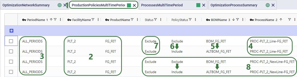
Lastly, the records that need to be added to the Production Policies Multi-Time Period table are the following 4 which have all the same values for the key columns as the 4 records in the above screenshot of the Production Policies single-period input table, which contain all the possible ways to produce FG_FET at PLT_2:
In the following example, we want to change the unit cost on 2 of the processes: at Plant 1 (PLT_1), the cost on the new potential line needs to be decreased to 0.005 for cheddar cheese (CHE) and increased to 0.015 for Swiss cheese (SWI). This can be done by using the Processes Multi-Time Period input table:
Note that there is also a Work Center Name field on the Processes Multi-Time Period table (not shown in the screenshot). As this is not a key field on the Processes input tables, it can be left blank here on the multi-time period table. This field will not be changed and the value from the single-time period table Work Center Name field will be used for these 2 records.
In the following example, we want to evaluate if upgrading the existing production lines at both plants from the 3rd year of the modelling horizon onwards, so they have a higher throughput capacity at a somewhat higher fixed operating cost, is a good alternative to opening one of the potential new lines at either plant. First, we add a new periods group to the model to set this up:
On the Groups table, we set up a new group named YEARS3-5 (Group Name) that is of Group Type = Periods and has 3 members: YEAR3, YEAR4 and YEAR5 (Member Name).
Cosmic Frog contains multiple tables through which different types of constraints can be added to network optimization (Neo) models. A constraint limits the model in a certain part of the network. These limits can for example be lower or upper limits in terms of the amount of flow between certain locations or certain echelons, the amount of inventory of a certain product or product group at a specific location or network wide, the amount of production of a certain product or product group at a specific location or network wide, etc. In this section the 3 constraints tables that are production specific will be covered: Production Constraints, Production Count Constraints, and Work Center Count Constraints.
A couple of general notes on all constraints tables:
In this example, we want to add constraints to the model that limit the production of all 5 finished goods together to 90,000 units. Both plants have this same upper production limit across the finished goods, and the limit applies to each year of the modelling horizon (5 yearly periods).
Note that there are more fields on the Production Constraints input table which are not shown in the above screenshot. These are:
In this example, we want to limit the number of products that are produced at PLT_1 to a maximum of 3 (out of the 5 finished goods). This limit applies over the whole 5-year modelling period, meaning that in total PLT_1 can produce no more than 3 finished goods:
Again, note there are more fields on the Production Count Constraints input table which are not shown in the above screenshot. These are:
Next, we will show an example of how to open at least 3 work centers, but no more than 5 out of 8 candidate work centers. These limits apply to all 5 yearly periods in the model together and over all facilities present in the model.
Again, there are more fields on the Work Center Count Constraints table that are not shown in the above screenshot:
After running a network optimization using Cosmic Frog’s Neo technology, production specific outputs can be found in several of the more general output tables, like the Optimization Network Summary, and the Optimization Constraints Summary (if any constraints were applied). Outputs more focused on just production can be found in 4 production specific output tables: the Optimization Production Summary, the Optimization Bills Of Material Summary, the Optimization Process Summary, and the Optimization Work Center Summary. We will cover these tables here, starting with the Optimization Network Summary.
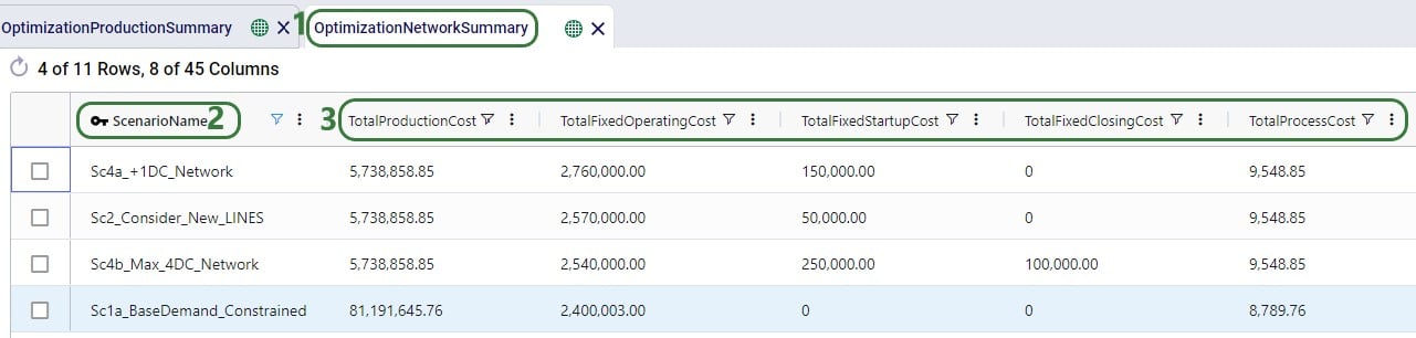
The following screenshot shows the production specific outputs that are contained in the Optimization Network Summary output table:
Other production related fields on this table which are not shown in the screenshot above are:
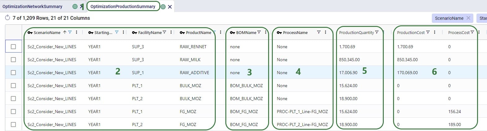
The Optimization Production Summary output table has a record with the production details for each product that was produced as part of the model run:
Other fields on this output table which are not shown in the screenshot are:
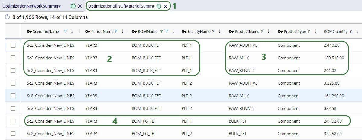
The details of how many components were used and how much by-product produced as a result of any bills of materials that were used as part of the production process can be found on the Optimization Bills Of Material Summary output table:
Note that aside from possibly knowing based on the BOM Name, it is not listed in the Bills Of Material Summary output table what the end product is and how much of it is produced as a result of a BOM. Those details are contained in the Optimization Production Summary output table discussed above.
Other fields on this output table which are not shown in the screenshot are:
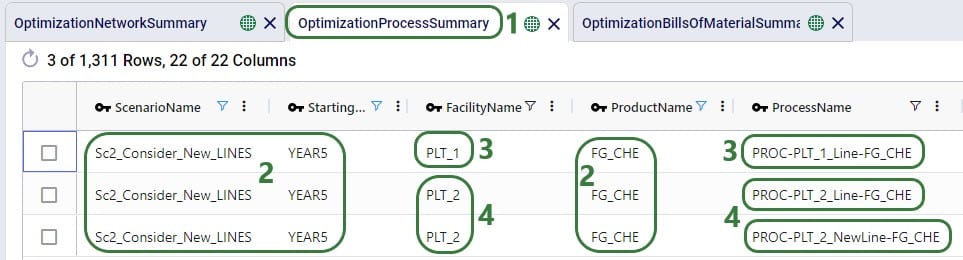
The details of all the steps of any processes used as part of the production in the Neo network optimization run can be found in the Optimization Process Summary, see these next 2 screenshots:
Other fields on this output table which are not shown in the screenshots are:
For each Work Center that has its Status set to Include or Consider, a record for each period of the model can be found in the Optimization Work Center Summary output table. It summarizes if the Work Center was used during that period, and, if so, how much and at what cost:
The following screenshot shows a few more output fields on the Optimization Work Center Summary output tables that have non-0 values in this model:
Other fields on this output table which are not shown in the screenshots are:
For all constraints in the model, the Optimization Constraint Summary can be a very handy table to check if any constraints are close to their maximum (or minimum, etc.) value to understand where the current and future bottlenecks are and likely will be. The screenshot below shows the outputs on this table for a production constraint that is applied at each of the 3 suppliers, where neither can produce more than 1 million units of RAW_MILK in any 1 year. In the screenshot we specifically look at the Supplier named SUP_3:
Other fields on this output table which are not shown in the screenshots are:
There are a few other output tables of which the main outputs are not related to production, but still contain several fields that result from productions. These are:
In this help article we have covered how to set up alternative Work Centers at existing locations and use the Work Center Status and Initial State fields to evaluate if including these, and from what period onwards if so, will be optimal. We have also covered how Work Center Count Constraints can be used to pick a certain amount of Work Centers to be opened/used from a set of multiple candidates, either at 1 location or multiple. Here we also want to mention that Facility Count Constraints can be used when making decisions at the plant level. Say that based on market growth in a certain region, a manufacturer decides a new plant needs to be built. There are 3 candidate locations for the plant from which the optimal needs to be picked. This can be set up as follows in Cosmic Frog:
A couple of alternative approaches to this are:
As mentioned above in the section on the Bill Of Materials input table, it is possible to set up a model where there is demand for a product that is the By-product resulting from a BOM. This does require some additional set up, and the below walks through this, while also showcasing how the model can be used to determine how much of any flexible demand for this by-product to fulfill. The screenshots show the set-up of a very simple example model built for this specific purpose.
On the Products table, besides the component (for which there also is demand in this model) that goes into any BOM, we also specify:
The demand for the 3 products is set up on the Customer Demand table and we notice that 1) there is demand for the Component, the End Product, and the By-Product, and 2) the Demand Status for ByProduct_1 is set to Consider, which means it does not need to be fulfilled, it will be (partially) fulfilled if it is optimal to do so. (For Component_1 and EndProduct_1 the Demand Status field is left blank, which means the default value of Include will be used.)
The EndProduct_1 is made through a BOM which consumes Component_1 and also make ByProduct_1 as a Byproduct. For this we need to set up a BOM:
Next, on the Production Policies table, we see that Component_1 can be created without a BOM, and:
In reality, these 2 production policies result in the same consumption of Component_1 and same production amounts of EndProduct_1 and ByProduct_1. Both need to be present however in order to be able to also have demand for ByProduct_1 in the model.
Other model elements that need to be set up are:
Three scenarios were run for this simple example model with the only difference between them the Unit Price for ByProduct_1: Baseline (price of ByProduct_1 = 3), PriceByproduct1 (Unit Price of ByProduct_1 = 1), PriceByproduct2 (Unit Price of ByProduct_1 = 2). Let’s review some of the outputs to understand how this Unit Price affects the fulfillment of the flexible demand for ByProduct_1:
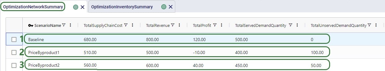
The high-level costs, revenues, profit and served/unserved demand outputs by scenario can be found on the Optimization Network Summary output table:
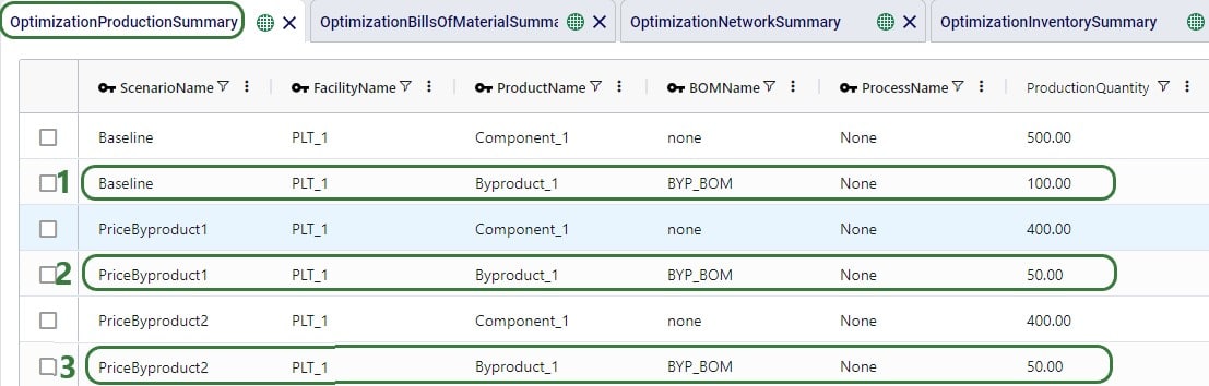
On the Optimization Production Summary output table, we see that all 3 scenarios used BYP_BOM for the production of EndProduct_1 and ByProduct_1, it could have also picked the other BOM (FG_BOM) and the overall results would have been the same.
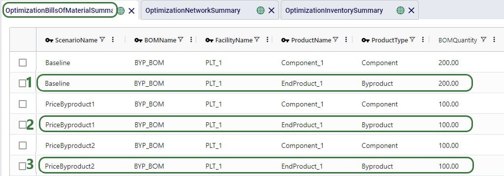
As the Optimization Production Summary only shows the production of the end products, we will also have a look at the Optimization Bills Of Material Summary output table:
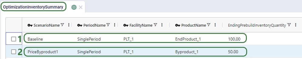
Lastly, we will have a look at the Optimization Inventory Summary output table:
Note that had the demand for Byproduct_1 been set to Include rather than Consider in this example model, all 3 scenarios would have produced 100 units of it to fulfill the demand, and as a result have produced 200 units of EndProduct_1. 100 of those would have been used to fulfill the demand for EndProduct_1 and the other 100 would have stayed in inventory, like we saw in the Baseline scenario above.