
The Supply Chain Decision Optimization Platform
Fast, AI-driven supply chain decision orchestration for every individual and team—from strategic design to tactical planning


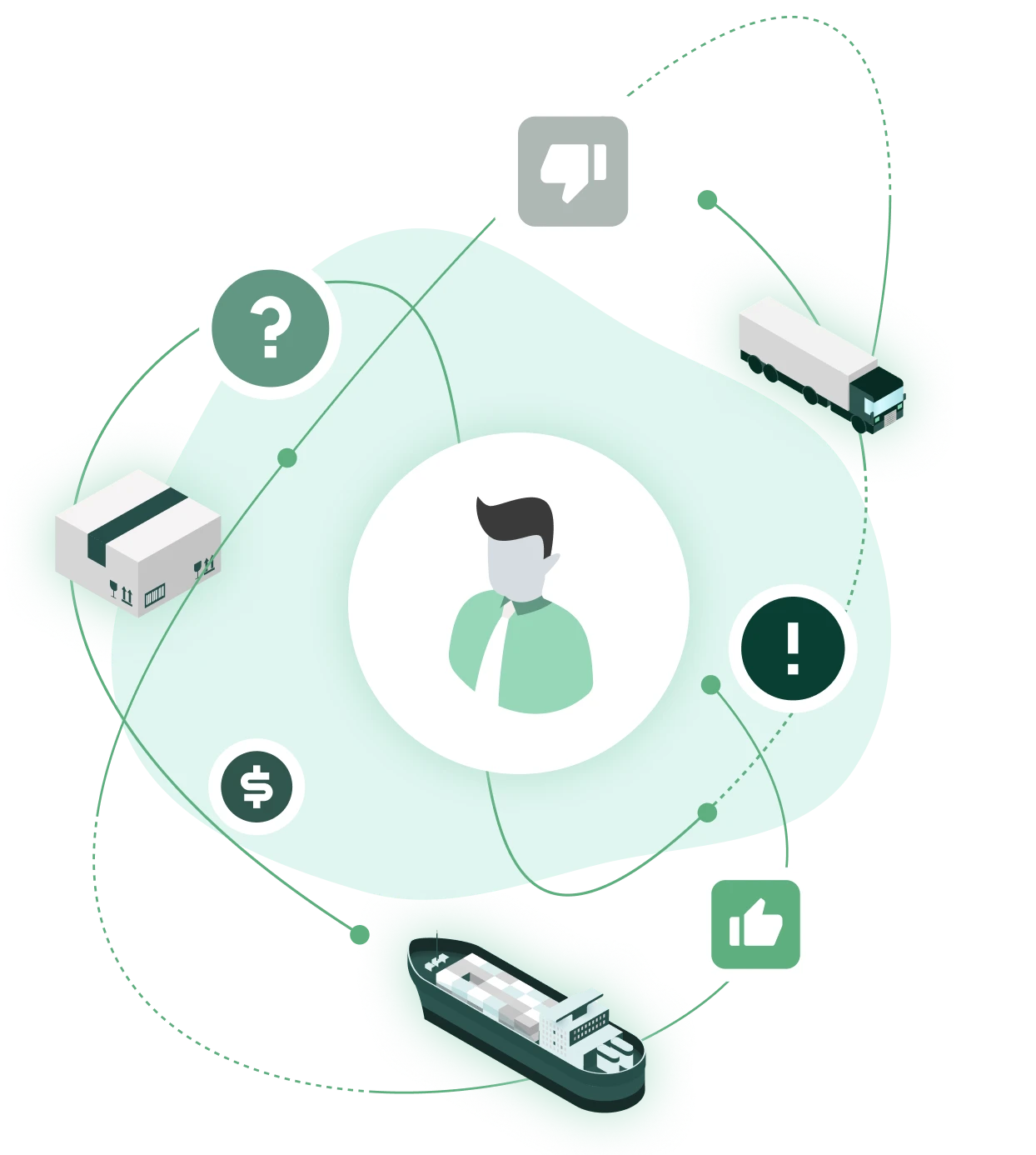
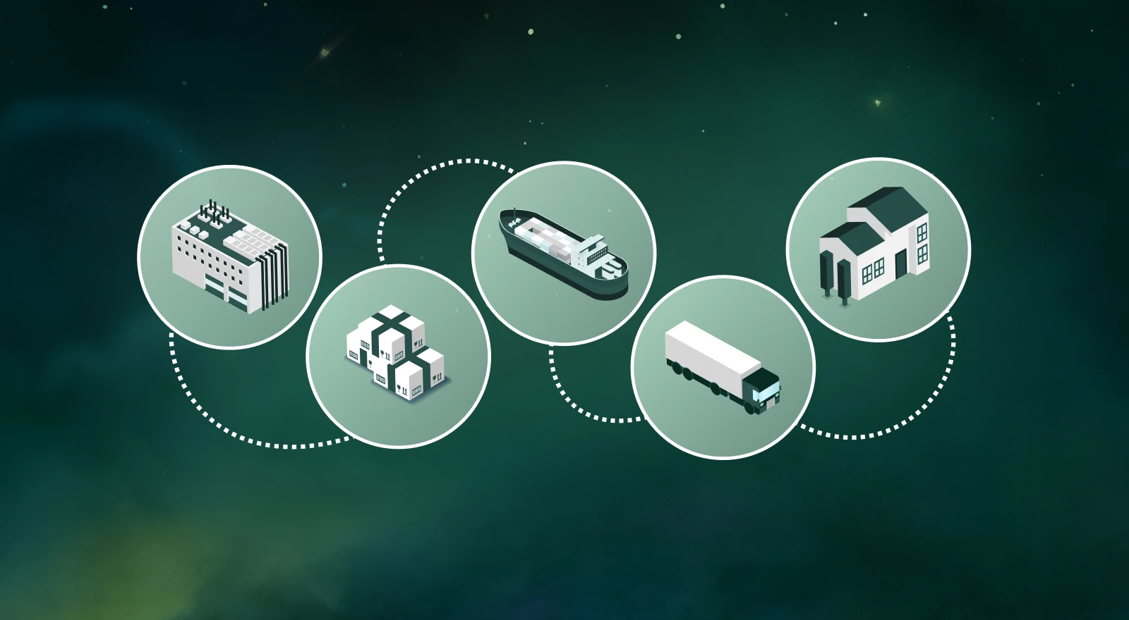
Answer any supply chain question—from big-picture to tactical and executional —across all supply chain functions


Decisions on facility locations, capacity investments, market expansion, demand planning and sales & operations planning

Evaluate sourcing strategies and tactical plans at the global, regional, and local levels.

Make smart decisions on facilities, inventory, outsourcing, and transportation

Drive ROI, resilience, and long-term value with data-driven supply chain decisions.

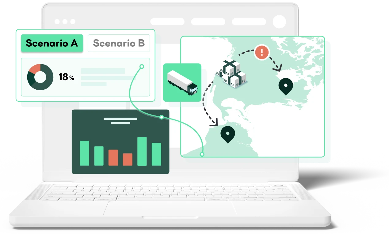
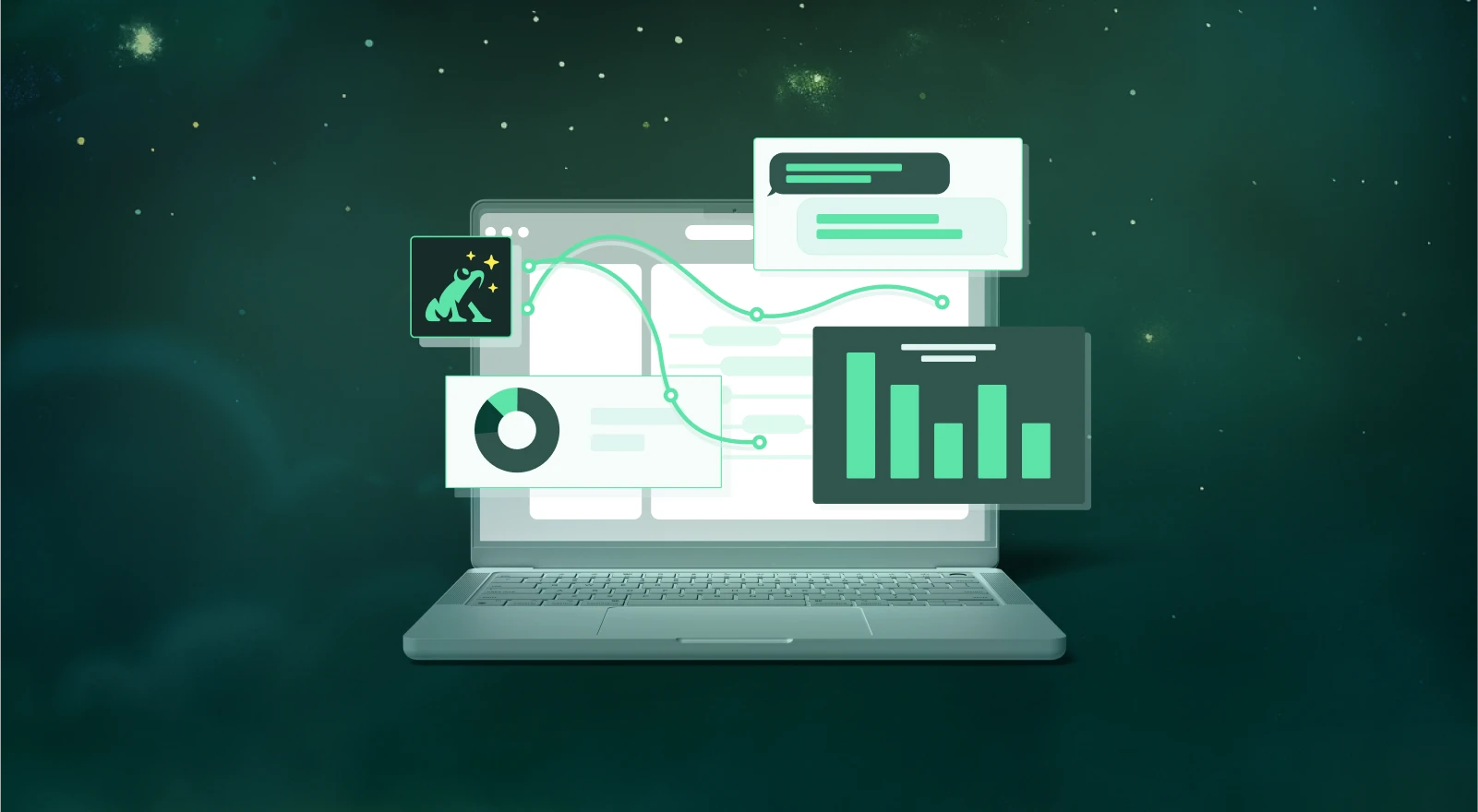
Quickly build, test, and refine supply chain scenarios with our intuitive cloud-based platform. .

Seamlessly connect and analyze supply chain data - unlock deeper insights and smarter supply chain decisions.

Get fast, optimized answers for even the trickiest tactical planning decisions.

Your people are your competitive advantage, but they're stuck with tools that can't keep up.
Supply chain practitioners face a barrage of decisions—cost, risk, resilience, sustainability—yet siloed systems, competing objectives, and delayed analysis make fast, confident action nearly impossible.
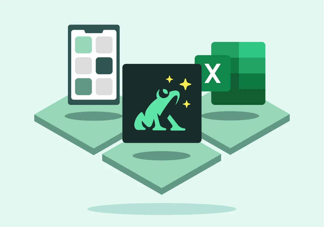
From strategic design to tactical planning, deliver optimization and AI decision-making power via Excel, google Sheets, and web and mobile apps your teams know and trust.
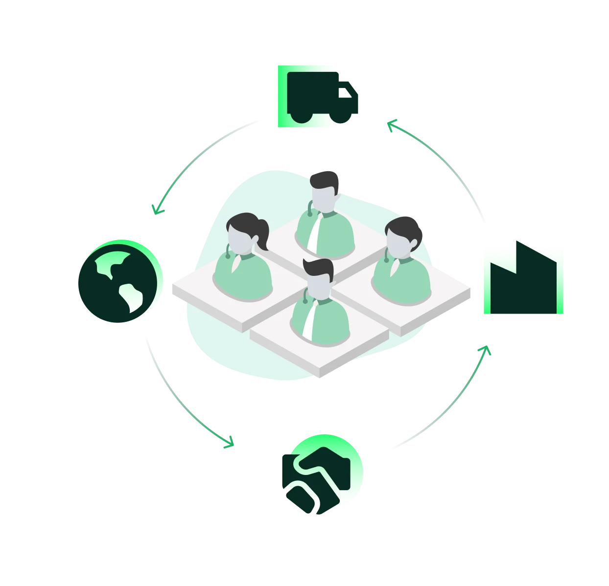
Align cross-functional teams and safely test and activate supply chain changes—faster and smarter.
Optimize future scenarios at enterprise scale. Only Optilogic enables you to plan proactively, respond to disruptions, and protect your P&L from the next wave of challenges.


No more modelers working in isolation or planning teams scrambling with tactical fire drills. We’re unifying design and planning into one seamless decision platform that puts optimization power directly in the hands of your people--whether you're optimizing a single route or redesigning your entire network.


SKU-level supply chain modeling and what-if scenarios with embedded AI, optimization, and simulation. One platform for strategic network design and tactical planning decisions—accessible through familiar spreadsheet interfaces and intuitive web and mobile apps.

AI and Agentic AI eliminates data challenges—autonomous cleansing and workflow orchestration delivers decision-ready intelligence instantly, so you can focus on making decisions, not wrangling data — resulting in faster time to insight.
Unlock enterprise collaboration and workflow automation that connects individuals, teams, and leadership in shared decision platform—breaking down silos between design and planning functions.
Get a live walkthrough of the platform with one of our experts.

.png)

.png)
Explore solutions built for every use case and industry—helping you overcome complex supply chain challenges with confidence.
The Optilogic Platform combines optimization, simulation, and secure data tools to solve enterprise-scale supply chain challenges with speed and flexibility.


