User-defined variables (UDVs) are a transformative feature in Cosmic Frog’s transportation optimization algorithm (Hopper engine) that allow users to create and track custom metrics specific to their transportation needs. Once established, these variables can be seamlessly integrated into user-defined constraints and/or user-defined costs. Several example use cases are:
Before diving into Hopper’s user-defined variables, costs, and constraints, it is recommended users are familiar with the basics of building and running a Hopper model, see for example this “Getting Started with Hopper” help center article.
In this documentation, we will first describe the example model used to illustrate the UDV concepts in this help article. Next, we will cover the input and output tables available when working with user-defined variables, costs, and constraints. Finally, we will walk through the inputs and outputs of 4 UDV examples: the first two examples showcase the application of constraints to user-defined variables, while the last two examples cover how to model user-defined costs.
The characteristics of the model used to show the concepts of user-defined variables, costs, and constraints throughout this help article are as follows:
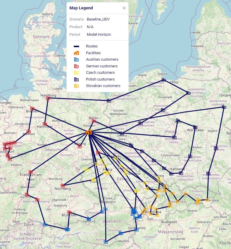
The optimized routes from the Baseline_UDV scenario are shown on this map, there are 10 routes with 10 stops each. The customers are color-coded based on the country they are in:
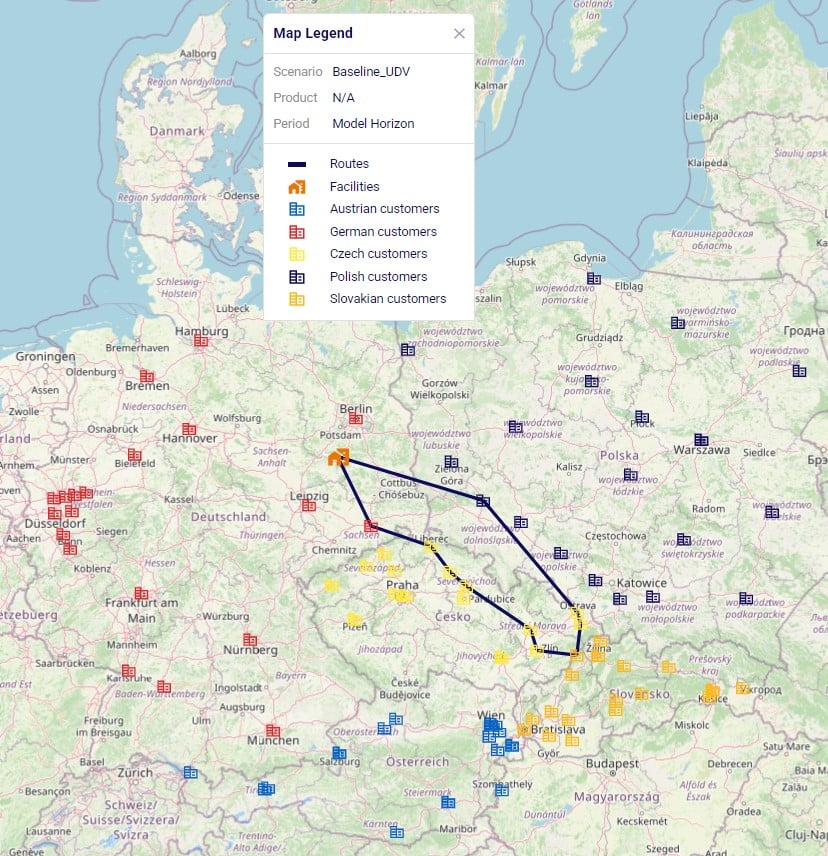
Filtering out the route which has stops in most countries, we find the following route which has stops on it in 4 countries Poland (1 dark blue stop), Czech Republic (7 yellow stops), Slovakia (1 orange stop), and Germany (1 red stop):
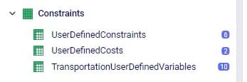
In the Input Tables part of Cosmic Frog’s Data module, there are 3 input tables in the Constraints section that can be used to configure user-defined variables, costs, and constraints:
We will take a closer look at each of these input tables now, and will also see more screenshots of these in the later sections that walk through several examples.
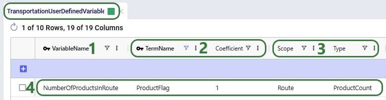
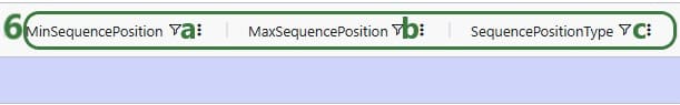
On this table we specify the term(s) of each variable which we wish to track or apply user-defined costs and/or constraints to. This first screenshot shows the fields which are used to define the variable, its term(s), and what the return condition is:
The next 2 screenshots show the other fields available on the Transportation User-Defined Variables input table, which are used to set the Filter Condition for the Scope. Note that several of these fields have accompanying Group Behavior fields, which are not shown in the screenshot. If a group name is used in the Asset Name, Site Name, Shipment ID, or Product Name field, the Group Behavior field specifies how the group should be interpreted: if the Group Behavior field is set to Aggregate (the default if not specified) the activity of the variable is summed over the members of the group, i.e. the variable is applied to the members of the group together. If the Group Behavior field is set to Enumerate, then an instance of the variable will be created for each member of the group individually.

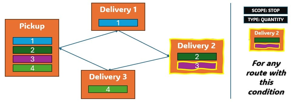
Consider a route which picks up 4 shipments, Shipment #1, #2, #3, and #4, and delivers them to 3 stops on a route as shown in the following diagram. In all 3 examples that follow, the filter condition is set to Shipment ID = Shipment #3 and Site Type = Delivery. This first example shows what will be returned for the variable when Scope = Shipment and Type = Quantity:

The whole route is filtered for Delivery of Shipment #3 and we see that it is delivered to the Delivery 2 stop. Since Scope = Shipment and Type = Quantity, the resulting variable value is the quantity of this shipment, which is what the yellow outline indicates.
In the next example, we look at the same route and same filtering condition (Shipment #3, Delivery), but now Scope has been changed to Stop (Type is still Quantity):
Again, we filter the route for Delivery of Shipment #3 and we see that it is delivered to the Delivery 2 stop. Since Scope = Stop, now the variable value is the total quantity delivered to the stop (outlined in yellow again): quantity Shipment #2 + quantity Shipment #3.
The final visual example is for when the Scope is now changed to Route, while keeping all the other settings the same:
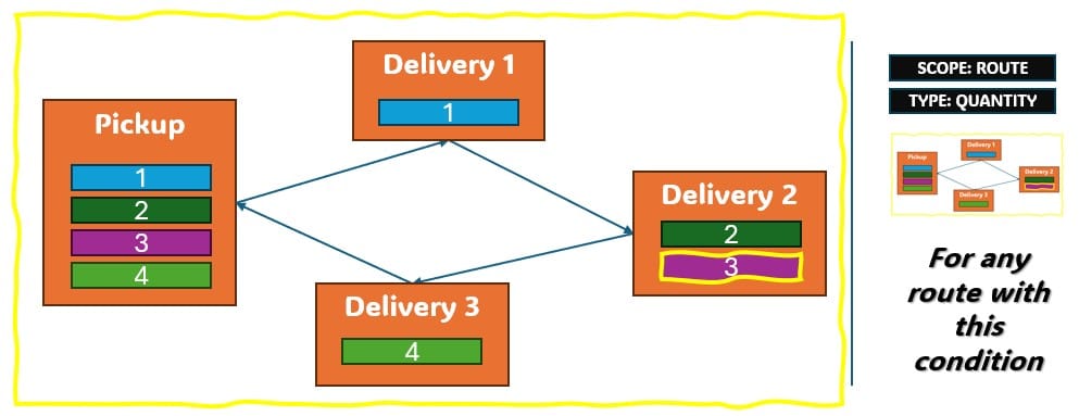
The route is again filtered for Delivery of Shipment #3, since the delivery of this shipment is on this route, we now calculate variable value as the total quantity of the route: quantity Shipment #1 + quantity Shipment #2 + quantity Shipment #3 + quantity Shipment #4, again outlined in yellow.
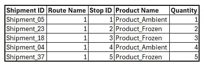
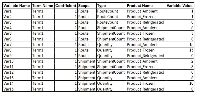
Next, we will also walk through a numbers example for different combinations of Scope and Type to see how these affect the calculation of the value of a variable’s term. Consider a route with 5 stops as follows:
We will calculate the value of the following 15 variables where the Scope, Type, and Product Name to filter for are set to different values. Note that all variables have just 1 term with coefficient 1, so the variable value = scaled term value.
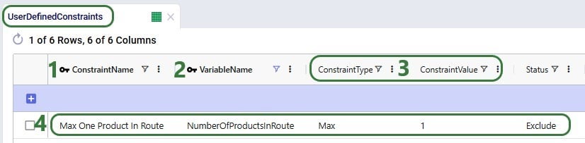
If wanting to apply constraints to user-defined variables, this can be set up on the User-Defined Constraints input table:
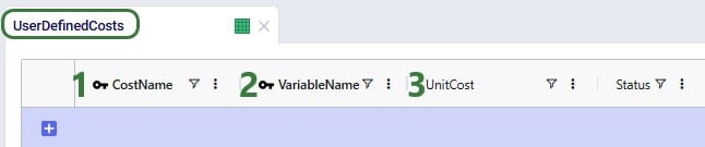
To apply costs to a user-defined variable, this can be achieved by utilizing the User-Defined Costs input table:
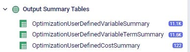
There are 3 output tables related to user-defined costs and constraints:
We will cover each of these now and will see more screenshots of them in the sections that follow where we will walk through several example use cases.
This table lists the values of the terms of each user-defined variable. This next screenshot shows the values of the “ProductFlag” term of the “NumberOfProductsInRoute” variable for the routes of the Baseline_UDV scenario. How this variable and its term were set up can be seen in the screenshot of the transportation user-defined variables table above (Scope = Route, Type = Product Count, Coefficient = 1).
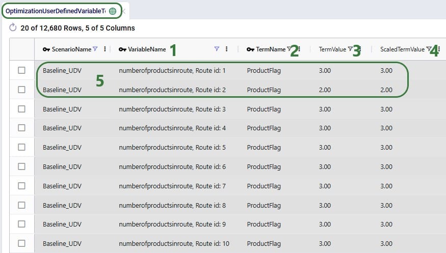
When setting up the Number Of Products In Route variable like above and not applying costs or constraints to it, it functions as a tracker so that user can easily get at this data rather than having to manipulate the transportation optimization output tables to calculate the number of products per route.
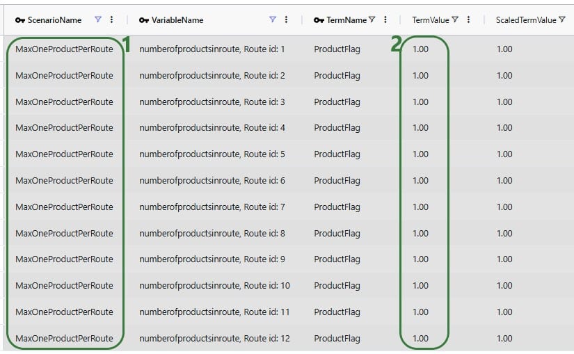
If we run a scenario “MaxOneProductPerRoute” where we include the maximum 1 product per route constraint that we have seen in the screenshot in the section further above on the User-Defined Constraints input table, the outputs in this table change as follows:
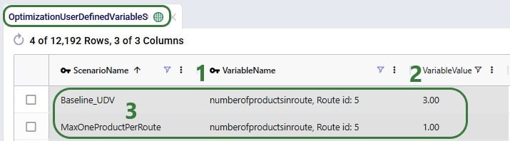
This table is a roll up to the variable level of the Optimization User-Defined Variable Term Summary output table discussed in the previous section. All the scaled terms of each variable have been added up to arrive at the variable’s value:
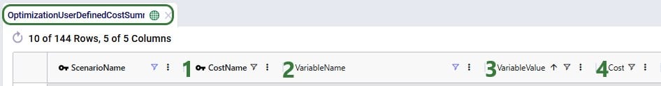
If costs have been applied to a user-defined variable, the results of that can be seen in this output table:
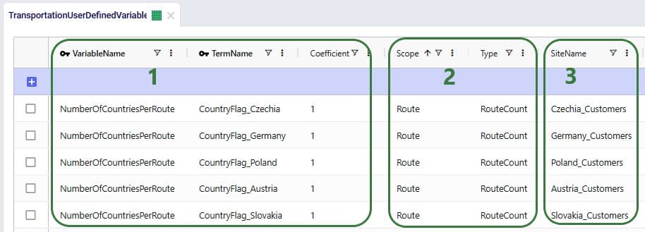
In this first example, we will see how we can track and limit the number of countries per route. For this purpose, a variable with 5 terms is set up in the Transportation User-Defined Variables table. Each term counts if a route has any stops in 1 of the 5 countries used in the model, 1 variable term for each country. Then we will apply constraints to this variable that limit the number of countries on each route to either 1 or 2. Let’s start with looking at the variable and its 5 terms in the Transportation User-Defined Variables table:
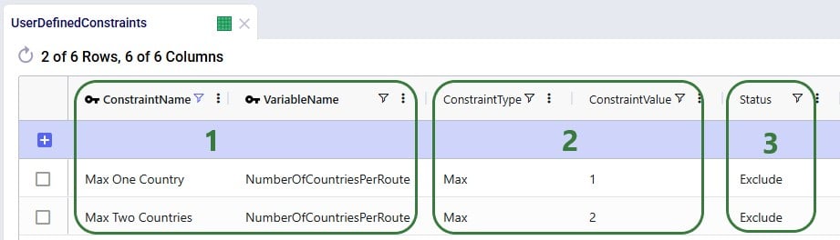
Next, we can add constraints that apply to this variable to change the behavior in the model and limit the number of countries a route is allowed to make stops in on any given route. We use the User-Defined Constraints table for this:
After running the Baseline_UDV scenario which does not include these constraints, we can have a look at the Optimization User-Defined Variable Summary output table:
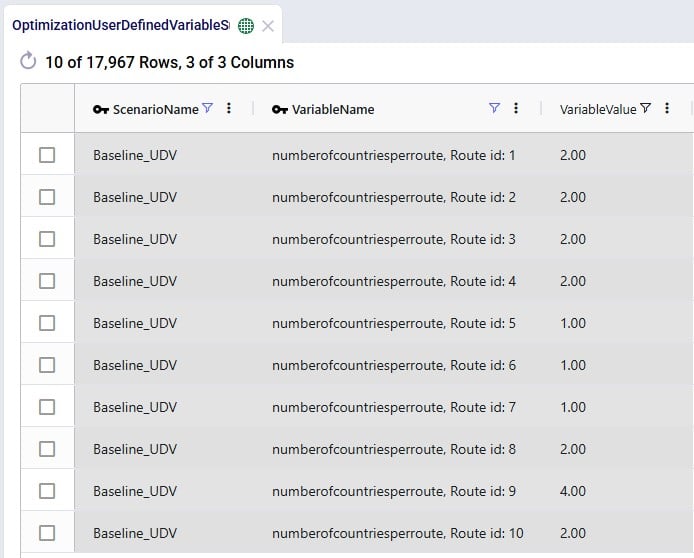
We see that 3 routes make stops in just 1 country, 5 routes in 2 countries, and 1 route (route 9) makes stops in 4 countries when leaving the number of countries a route is allowed to make stops in unconstrained.
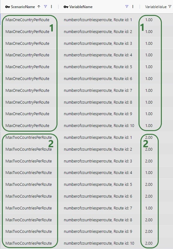
Now we want to see the impact of applying the Max One Country and Max Two Countries constraints through 2 scenarios and again we check the Optimization User-Defined Variable Summary output table after running these scenarios:
Maps are also helpful to visualize these outputs. As we saw in the introduction of the example model used throughout this documentation, these are the Baseline_UDV routes visualized on a map:
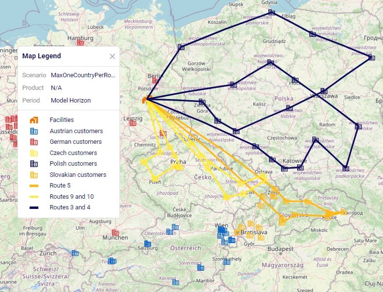
These routes change as follows in the MaxOneCountryPerRoute scenario:

Since some of these routes overlap on the map, let us filter a few out and color-code them based on the country to more easily see that indeed the routes each only make stops in 1 country:
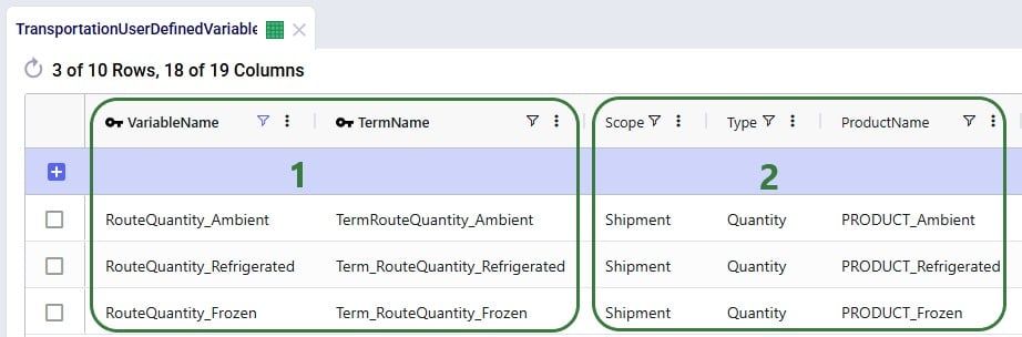
In this example we will see how user-defined variables and constraints can be used to model truck compartments and their capacities. First, we set up 3 variables that track the amount of ambient, refrigerated, and frozen product on a route:
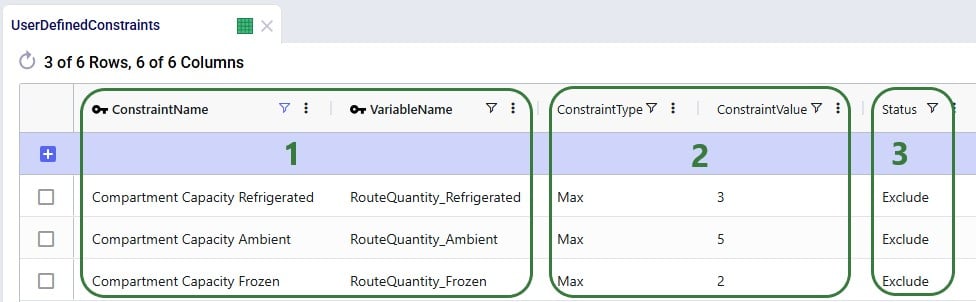
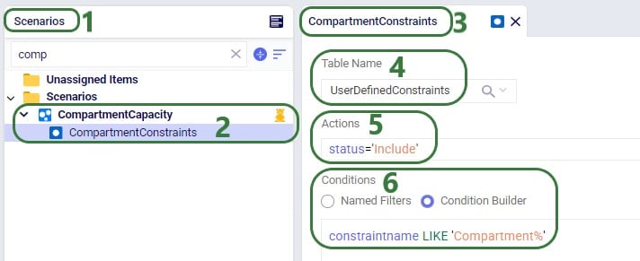
Without setting up any constraints that apply to these variables, they just track how much of each product is on a route, which can be within or over the actual compartment capacity. So, to set capacity limits, we can use the User-Defined Constraints table to setup constraints on these 3 variables that represent the capacity of the ambient, refrigerated, and frozen compartments of a truck:
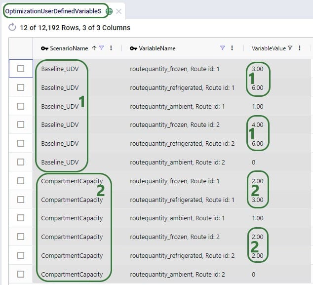
After running the Baseline_UDV scenario where these constraints are not applied and another scenario, Compartment Capacity, where they are applied, we can take a look at the Optimization User-Defined Variable Summary output table to see the effect of the constraints (just showing routes 1 and 2 in the below screenshot):
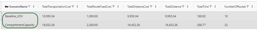
Typically, when adding constraints, we expect routes to change – more routes may be needed to adhere to the constraints, and they may become less efficient. Overall, we would expect costs, distance, and time to increase. This is exactly what we see when comparing these outputs in the Transportation Summary output table for these 2 scenarios:
We have seen 2 examples of applying constraints to user-defined variables in the previous sections. Now, we will walk through 2 examples of applying costs to user-defined variables. The first example shows how to apply a variable cost based on how long a shipment sits on a route: we will specify a cost of $1 per hour the shipment spends on the route. First, we set up a variable that tracks how long a shipment spends on a route in the Transportation User-Defined Variables input table:

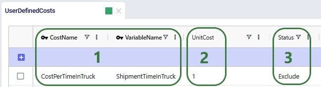
Next, the User-Defined Costs table is used to specify the cost of $1 per hour:
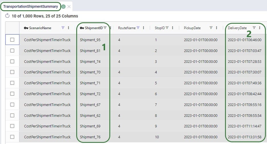
After running the CostPerShipmentTimeInTruck scenario which includes this user-defined cost, we can look at both the Transportation Shipment Summary and the Optimization User-Defined Cost Summary output tables to see this cost of $1 per hour has been applied:
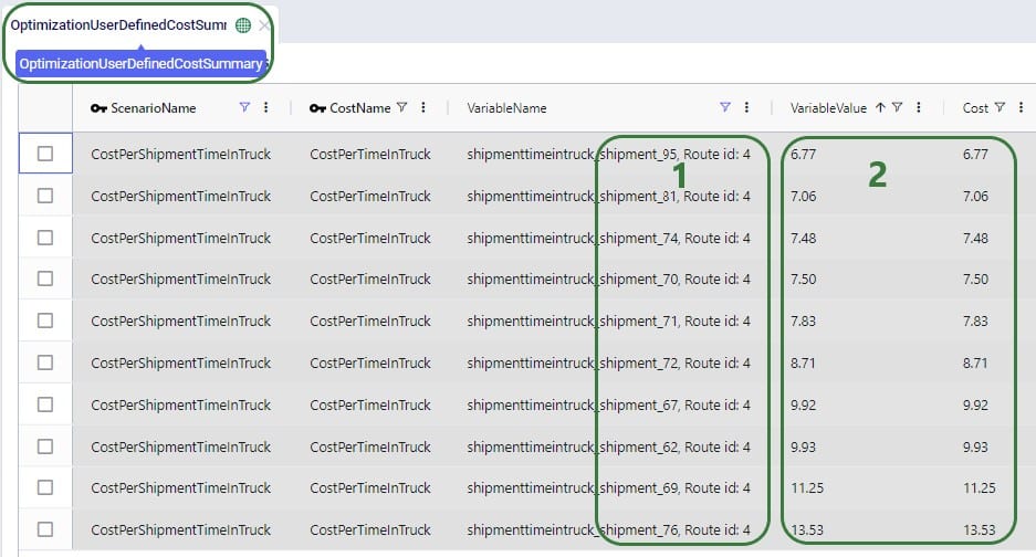
Next, we open the Optimization User-Defined Cost Summary output table and filter for the same scenario and route (#4):
In our final example of this documentation, we will use the same variable ShipmentTimeInTruck from the previous example to set up a different type of cost. We will use it to find any shipments that are on a route for more than 10 hours and apply a penalty cost of $100 to each. This involves using a step cost for which we will also need to utilize the Step Costs table; we will start with looking at this table:
Next, we configure the penalty cost in the User-Defined Costs table:
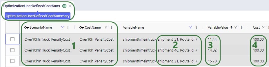
After running a scenario in which we include the penalty cost, we can again look at the Transportation Shipment Summary and Optimization User-Defined Cost Summary output tables to see this cost in action:

User-defined variables (UDVs) are a transformative feature in Cosmic Frog’s transportation optimization algorithm (Hopper engine) that allow users to create and track custom metrics specific to their transportation needs. Once established, these variables can be seamlessly integrated into user-defined constraints and/or user-defined costs. Several example use cases are:
Before diving into Hopper’s user-defined variables, costs, and constraints, it is recommended users are familiar with the basics of building and running a Hopper model, see for example this “Getting Started with Hopper” help center article.
In this documentation, we will first describe the example model used to illustrate the UDV concepts in this help article. Next, we will cover the input and output tables available when working with user-defined variables, costs, and constraints. Finally, we will walk through the inputs and outputs of 4 UDV examples: the first two examples showcase the application of constraints to user-defined variables, while the last two examples cover how to model user-defined costs.
The characteristics of the model used to show the concepts of user-defined variables, costs, and constraints throughout this help article are as follows:
The optimized routes from the Baseline_UDV scenario are shown on this map, there are 10 routes with 10 stops each. The customers are color-coded based on the country they are in:
Filtering out the route which has stops in most countries, we find the following route which has stops on it in 4 countries Poland (1 dark blue stop), Czech Republic (7 yellow stops), Slovakia (1 orange stop), and Germany (1 red stop):
In the Input Tables part of Cosmic Frog’s Data module, there are 3 input tables in the Constraints section that can be used to configure user-defined variables, costs, and constraints:
We will take a closer look at each of these input tables now, and will also see more screenshots of these in the later sections that walk through several examples.
On this table we specify the term(s) of each variable which we wish to track or apply user-defined costs and/or constraints to. This first screenshot shows the fields which are used to define the variable, its term(s), and what the return condition is:
The next 2 screenshots show the other fields available on the Transportation User-Defined Variables input table, which are used to set the Filter Condition for the Scope. Note that several of these fields have accompanying Group Behavior fields, which are not shown in the screenshot. If a group name is used in the Asset Name, Site Name, Shipment ID, or Product Name field, the Group Behavior field specifies how the group should be interpreted: if the Group Behavior field is set to Aggregate (the default if not specified) the activity of the variable is summed over the members of the group, i.e. the variable is applied to the members of the group together. If the Group Behavior field is set to Enumerate, then an instance of the variable will be created for each member of the group individually.
Consider a route which picks up 4 shipments, Shipment #1, #2, #3, and #4, and delivers them to 3 stops on a route as shown in the following diagram. In all 3 examples that follow, the filter condition is set to Shipment ID = Shipment #3 and Site Type = Delivery. This first example shows what will be returned for the variable when Scope = Shipment and Type = Quantity:
The whole route is filtered for Delivery of Shipment #3 and we see that it is delivered to the Delivery 2 stop. Since Scope = Shipment and Type = Quantity, the resulting variable value is the quantity of this shipment, which is what the yellow outline indicates.
In the next example, we look at the same route and same filtering condition (Shipment #3, Delivery), but now Scope has been changed to Stop (Type is still Quantity):
Again, we filter the route for Delivery of Shipment #3 and we see that it is delivered to the Delivery 2 stop. Since Scope = Stop, now the variable value is the total quantity delivered to the stop (outlined in yellow again): quantity Shipment #2 + quantity Shipment #3.
The final visual example is for when the Scope is now changed to Route, while keeping all the other settings the same:
The route is again filtered for Delivery of Shipment #3, since the delivery of this shipment is on this route, we now calculate variable value as the total quantity of the route: quantity Shipment #1 + quantity Shipment #2 + quantity Shipment #3 + quantity Shipment #4, again outlined in yellow.
Next, we will also walk through a numbers example for different combinations of Scope and Type to see how these affect the calculation of the value of a variable’s term. Consider a route with 5 stops as follows:
We will calculate the value of the following 15 variables where the Scope, Type, and Product Name to filter for are set to different values. Note that all variables have just 1 term with coefficient 1, so the variable value = scaled term value.
If wanting to apply constraints to user-defined variables, this can be set up on the User-Defined Constraints input table:
To apply costs to a user-defined variable, this can be achieved by utilizing the User-Defined Costs input table:
There are 3 output tables related to user-defined costs and constraints:
We will cover each of these now and will see more screenshots of them in the sections that follow where we will walk through several example use cases.
This table lists the values of the terms of each user-defined variable. This next screenshot shows the values of the “ProductFlag” term of the “NumberOfProductsInRoute” variable for the routes of the Baseline_UDV scenario. How this variable and its term were set up can be seen in the screenshot of the transportation user-defined variables table above (Scope = Route, Type = Product Count, Coefficient = 1).
When setting up the Number Of Products In Route variable like above and not applying costs or constraints to it, it functions as a tracker so that user can easily get at this data rather than having to manipulate the transportation optimization output tables to calculate the number of products per route.
If we run a scenario “MaxOneProductPerRoute” where we include the maximum 1 product per route constraint that we have seen in the screenshot in the section further above on the User-Defined Constraints input table, the outputs in this table change as follows:
This table is a roll up to the variable level of the Optimization User-Defined Variable Term Summary output table discussed in the previous section. All the scaled terms of each variable have been added up to arrive at the variable’s value:
If costs have been applied to a user-defined variable, the results of that can be seen in this output table:
In this first example, we will see how we can track and limit the number of countries per route. For this purpose, a variable with 5 terms is set up in the Transportation User-Defined Variables table. Each term counts if a route has any stops in 1 of the 5 countries used in the model, 1 variable term for each country. Then we will apply constraints to this variable that limit the number of countries on each route to either 1 or 2. Let’s start with looking at the variable and its 5 terms in the Transportation User-Defined Variables table:
Next, we can add constraints that apply to this variable to change the behavior in the model and limit the number of countries a route is allowed to make stops in on any given route. We use the User-Defined Constraints table for this:
After running the Baseline_UDV scenario which does not include these constraints, we can have a look at the Optimization User-Defined Variable Summary output table:
We see that 3 routes make stops in just 1 country, 5 routes in 2 countries, and 1 route (route 9) makes stops in 4 countries when leaving the number of countries a route is allowed to make stops in unconstrained.
Now we want to see the impact of applying the Max One Country and Max Two Countries constraints through 2 scenarios and again we check the Optimization User-Defined Variable Summary output table after running these scenarios:
Maps are also helpful to visualize these outputs. As we saw in the introduction of the example model used throughout this documentation, these are the Baseline_UDV routes visualized on a map:
These routes change as follows in the MaxOneCountryPerRoute scenario:
Since some of these routes overlap on the map, let us filter a few out and color-code them based on the country to more easily see that indeed the routes each only make stops in 1 country:
In this example we will see how user-defined variables and constraints can be used to model truck compartments and their capacities. First, we set up 3 variables that track the amount of ambient, refrigerated, and frozen product on a route:
Without setting up any constraints that apply to these variables, they just track how much of each product is on a route, which can be within or over the actual compartment capacity. So, to set capacity limits, we can use the User-Defined Constraints table to setup constraints on these 3 variables that represent the capacity of the ambient, refrigerated, and frozen compartments of a truck:
After running the Baseline_UDV scenario where these constraints are not applied and another scenario, Compartment Capacity, where they are applied, we can take a look at the Optimization User-Defined Variable Summary output table to see the effect of the constraints (just showing routes 1 and 2 in the below screenshot):
Typically, when adding constraints, we expect routes to change – more routes may be needed to adhere to the constraints, and they may become less efficient. Overall, we would expect costs, distance, and time to increase. This is exactly what we see when comparing these outputs in the Transportation Summary output table for these 2 scenarios:
We have seen 2 examples of applying constraints to user-defined variables in the previous sections. Now, we will walk through 2 examples of applying costs to user-defined variables. The first example shows how to apply a variable cost based on how long a shipment sits on a route: we will specify a cost of $1 per hour the shipment spends on the route. First, we set up a variable that tracks how long a shipment spends on a route in the Transportation User-Defined Variables input table:
Next, the User-Defined Costs table is used to specify the cost of $1 per hour:
After running the CostPerShipmentTimeInTruck scenario which includes this user-defined cost, we can look at both the Transportation Shipment Summary and the Optimization User-Defined Cost Summary output tables to see this cost of $1 per hour has been applied:
Next, we open the Optimization User-Defined Cost Summary output table and filter for the same scenario and route (#4):
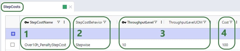
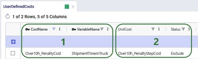
In our final example of this documentation, we will use the same variable ShipmentTimeInTruck from the previous example to set up a different type of cost. We will use it to find any shipments that are on a route for more than 10 hours and apply a penalty cost of $100 to each. This involves using a step cost for which we will also need to utilize the Step Costs table; we will start with looking at this table:
Next, we configure the penalty cost in the User-Defined Costs table:
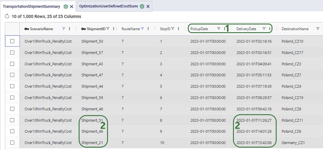
After running a scenario in which we include the penalty cost, we can again look at the Transportation Shipment Summary and Optimization User-Defined Cost Summary output tables to see this cost in action: