Exciting new features which enable users to solve both network and transportation optimization in one solve have been added to Cosmic Frog. By optimizing multi-stop route optimization as part of Network Optimization, it enables users to streamline their analysis and make their Network Optimization more accurate. This is possible because the single optimization solve calculates multi-stop route costs by shipment/customer combination, uses this cost as part of another possible transportation mode in addition to OTR, Rail, Air, etc. and will result in more accurate answers by including better transportation costs in a single solve.
In addition to this documentation, these 2 videos cover the new Network Transportation Optimization (NTO) features too:
Network Transportation Optimization is particularly useful for two classic network design problems (both will be described in more detail in the next section):
This feature set includes 2 ways of running the Transportation Optimization (Hopper) and Network Optimization (Neo) engines together:
Following will be covered in this documentation for both the Hopper within Neo and Hopper after Neo NTO algorithms: example use cases, model inputs, how to use the new features, basics of the model used to show the NTO features, and walk through 2 example models, including their setup (input tables, scenarios), and analysis of the outputs using tables and maps.
With this feature, users can consider routes as inputs in a Neo model, meaning that the model will optimize product flow sources based on all costs, including the cost of routes. Costs and asset capacities are taken into account for the routes.
Two example use cases which can be addressed using Hopper within Neo are customer consolidation and hub optimization, which will be illustrated with the images that follow.
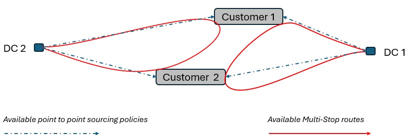
Consider a network where 2 distribution centers (DCs) are available to serve the customers. Two of these customers are in between the DCs and can either be serviced by the DCs directly (the blue dashed point to point lines) or product can be delivered to both of them as part of a multi-stop route from either DC (the red solid lines):
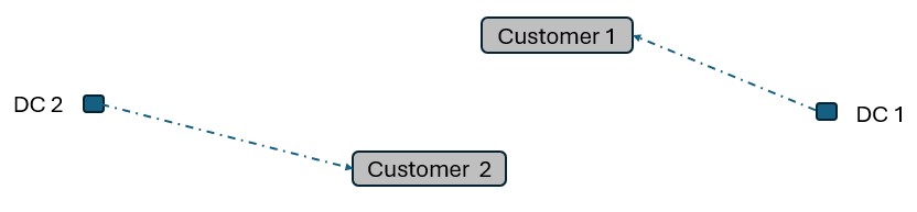
Running Neo without Hopper, not taking any route inputs into account, can lead to a solution where each DC serves 1 customer:
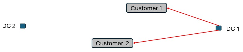
Whereas when taking route costs and capacities into account during a Hopper within Neo solve, it may be found that the overall cost solution is lower if one of the DCs (DC 1 in this example) serves both customers using a multi-stop route:
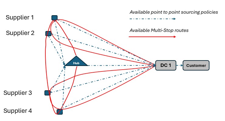
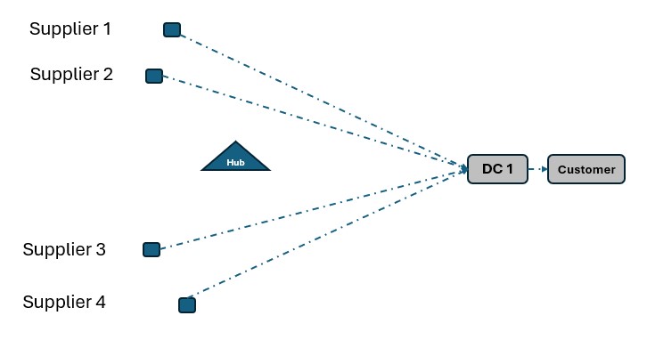
As a second example, consider a network where Suppliers can either deliver product to a Hub, either direct or on a multi-stop route from multiple suppliers, or direct/on multi-stop routes from multiple suppliers to a Distribution Center. Again, blue dashed lines indicate direct point to point deliveries and red lines indicate multi-stop route options:
Not taking route options into account when running Neo without Hopper can lead to a solution where each Supplier delivers to DC 1 directly:
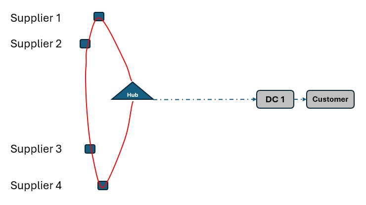
This solution can change to one where the Suppliers deliver to the Hub on a multi-stop route when taking the route options into account in a Neo within Hopper run if this is overall beneficial (e.g. lower total cost) to do:
The Hopper within Neo algorithm needs inputs in order to consider routes as part of the Neo network optimization run. These include:
In all cases, additional records need to be added to the Transportation Policies table as well (explained in more detail below), and if the Transit Matrix table is populated, it will also be used for Hopper within Neo runs.
Please note that any other Hopper related tables (e.g. relationship constraints, business hours, transportation stop rates, etc.), whether populated or not, are not used during a Hopper within Neo solve.
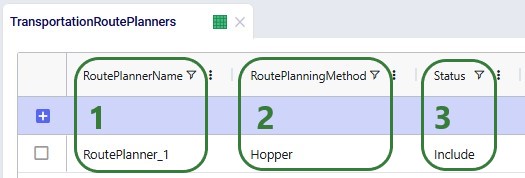
To use the Hopper algorithm for route generation, the Transportation Route Planners table and Transportation Policies tables need to be used. Starting with the Transportation Route Planners table:
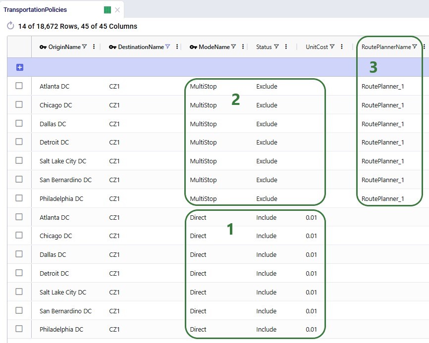
In the Transportation Policies table, records need to be added to indicate which lanes will be considered to be part of a multi-stop route:
Under the hood, potential routes will be calculated based on the inputs provided by the user. For example, for a case where the shipments table is not populated, and the user has specified their own assets:
As a numbers example to illustrate this calculation of a candidate route, let us consider following:
These costs are then used as inputs into the Network Optimization, together with costs for other transportation modes, and all are taken into account when optimizing the model.
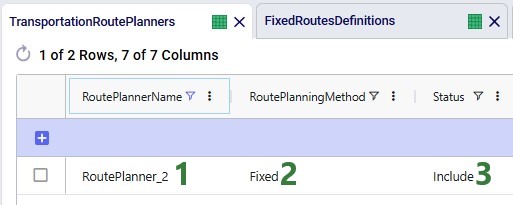
To use routes that are defined by the user in the Neo solve, the user also needs to use the Transportation Route Planners table, in combination with the Fixed Routes, Fixed Routes Definitions, and Transportation Policies tables. Starting with the Transportation Route Planners table:
The Fixed Routes table connects the names of the routes the user defines with the route planner name:
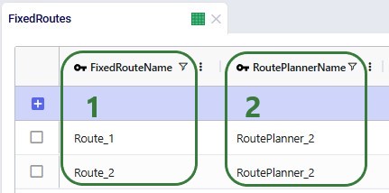
There are a few additional columns on the Fixed Routes table which are not shown in the screenshot above. These are:
The Fixed Routes Definitions table needs to be used to indicate which stops are on a route together:
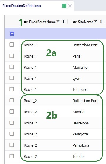
Please note that the Stop Number field on this table is currently not used by the Hopper within Neo functionality. The solve will determine the sequence of the stops.
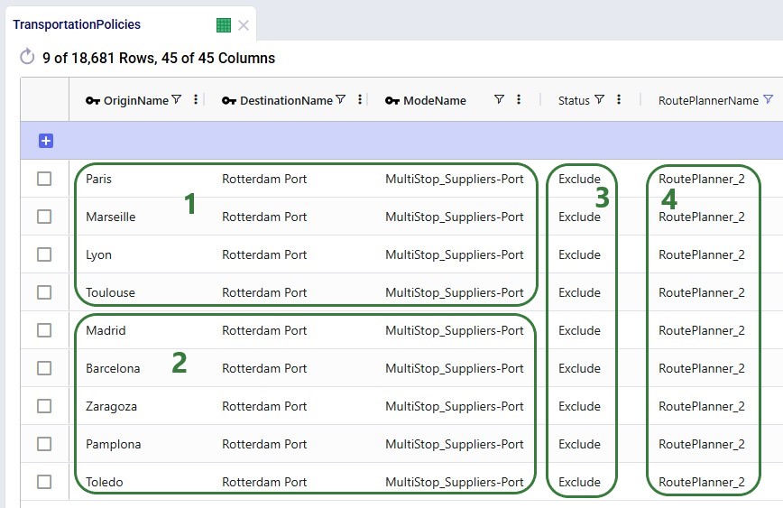
Finally, to understand which locations function as sources (pickups) and which as drop-offs (deliveries) on a route, and to indicate that multi-stop routes are an option for these source-destination combinations, corresponding records need to be added to the transportation policies table too:
A copy of the Global Supply Chain Strategy model from the Resource Library was used as the starting point for both the Hopper within Neo and Hopper after Neo demo models. The original Global Supply Chain Strategy model can be found here on the Resource Library, and a video describing it can be found in this "Global Supply Chain Strategy Demo Model Review" Help Center article. The modified models showing the Hopper within and after Neo functionality can be found here on the Resource Library:
To learn more about the Resource Library and how to use it, please see the "How to use the Resource Library" Help Center article.
A short description of the main elements in this model is as follows:
We illustrate the locations and flow of product through the following 3 maps:
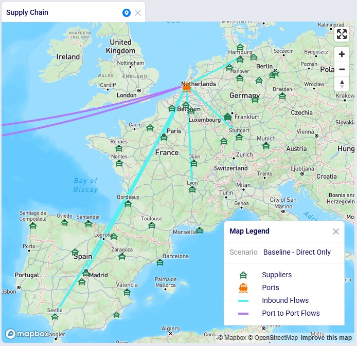
Even though around 35 suppliers are set up in the model in the EMEA region, only 6 of them are used based on the records in the Supplier Capabilities input table. We see the light blue lines from these suppliers delivering raw materials to the port in Rotterdam. From there, the 2 purple lines indicate the transport of the raw materials from Rotterdam to the US and Mexican ports.
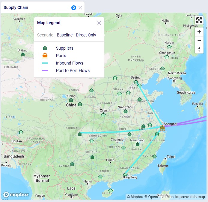
Similarly, around 35 suppliers are set up in China in the model, but only 3 of them are used per the set up in the Supplier Capabilities input table. The light blue lines are the transport of raw materials from the suppliers to the Shanghai port and the purple lines from the Shanghai port to the ports in Mexico and the US.
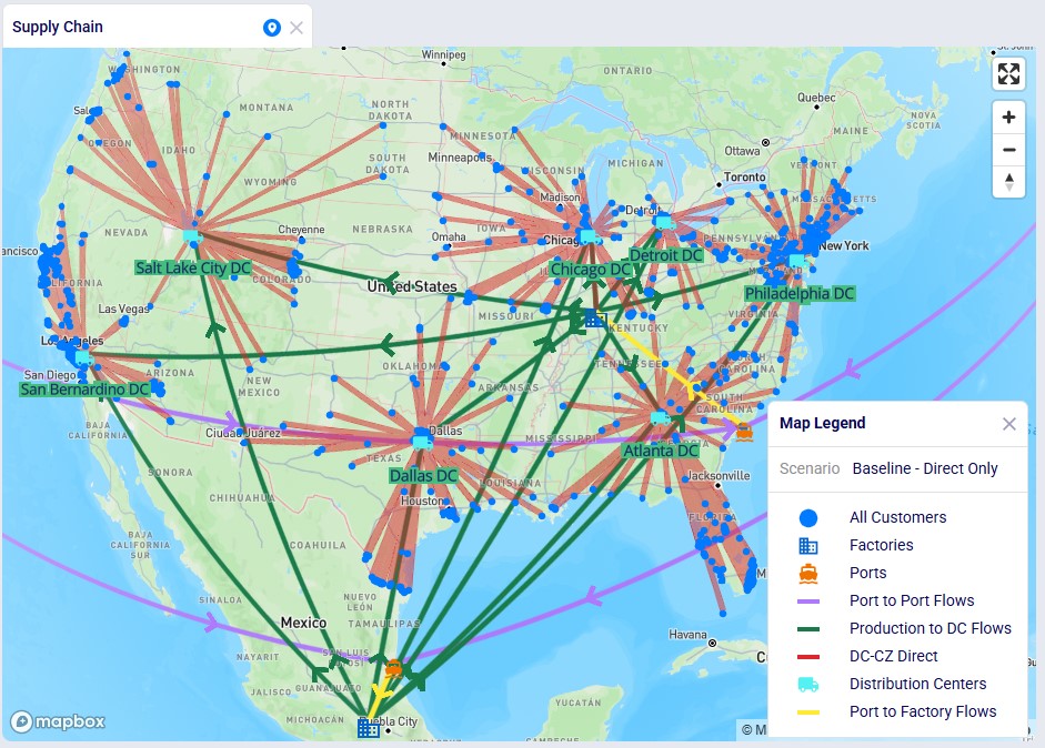
This map shows the flows into and within/between the US and Mexico locations:
We will show how Hopper routes for the last leg of the network, from DCs to customers, can be taken into account during a Neo solve. Through a series of scenarios, we will explore if using multi-stop routes for this supply chain is beneficial:
After copying the Global Supply Chain Strategy model from the Resource Library, following changes/additions were made to be able to consider Hopper generated routes for the DC-CZ leg during the Neo solve. After listing these changes here, we will explain each in more detail through screenshots further below. Users can copy this modified model with the scenarios, outputs, and preconfigured maps from the Resource Library.
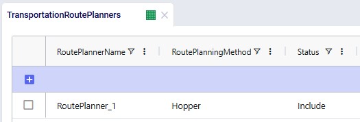
One record is added in this table where it is indicated that the route planner named "RoutePlanner_1" will use Hopper generated routes and is by default included during a Neo solve.
We choose to add our own asset instead of the 3 defaults ones that will be used if the Transportation Assets table is left blank. The characteristics of our large vehicle are shown in the next 2 screenshots:
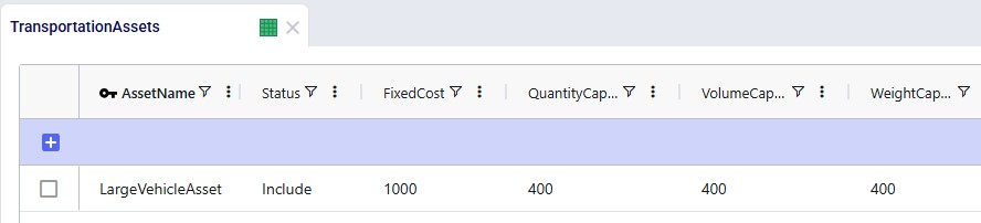
This large asset is included in the scenario runs as its Status = Include. The fixed cost of the asset is $1,000, with a capacity of 400 units / 400 cubic feet / 400 pounds.
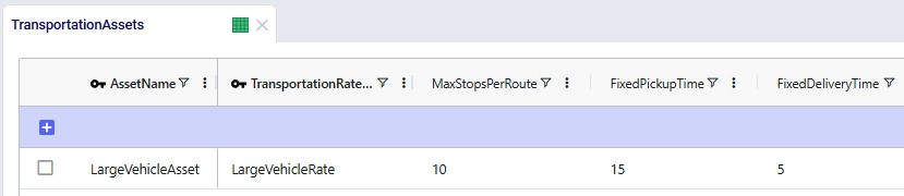
A rate record is set up in the Transportation Rates input table in order to model distance- and time-based costs. This is shown in the next screenshot. To use it, we link it to the asset by using the Transportation Rate Name field on the Transportation Assets table.
The Max Stops Per Route is set to 10. A Fixed Pickup Time of 15 minutes is entered, which will be applied once when picking up product at the DCs. Also, a Fixed Delivery Time of 5 minutes is set, this will be applied once at each customer when delivering product (the UOM fields are omitted in the screenshot; they are set to MIN).
Besides the fixed cost for the asset as specified in the Transportation Assets table, we also want to apply both distance- and time-based costs to the routes:
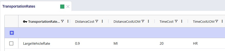
A record is set up in the Transportation Rates table where Transportation Rate Name is used in the Transportation Assets table to link the correct rate to the correct asset (e.g. LargeVehicleRate is used for the LargeVehicleAsset). The per distance cost is set to 0.9 per mile, and the time cost is set to 20 per hour; the latter mostly reflects the cost for the driver.
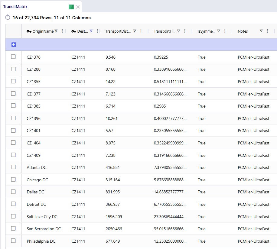
For the scenarios to use actual road distances and transport times, the Distance Lookup Utility in Cosmic Frog was used with following parameters:
A subset of records filtered for 1 customer destination (CZ1411) is shown in this next screenshot where we see the distance and time from the 10 closest other customers to this customer, and also from all 7 DCs:
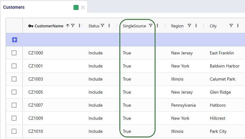
To remove potential dual sourcing, all customers are set to single sourcing (Single Source field is set to True on the Customers table), meaning they need to be served all product they demand from a single DC. In this model, setting customers to single sourcing also helps reduce the runtime of the scenarios:
To further help reduce solve times, a flow count constraint that allows the selection of at maximum 1 mode to each customer is added:
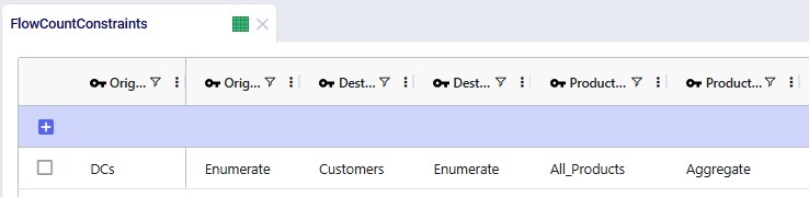
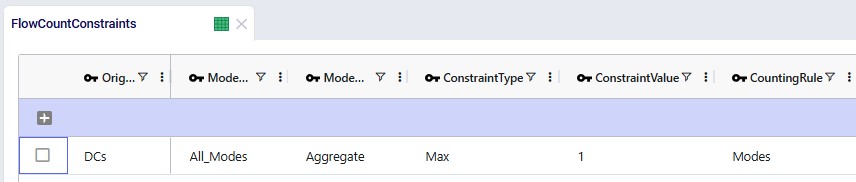
Groups for all DCs, all Customers, all Products, and all Modes (the 2 to customers, Direct and MultiStop) are being used in the Origin, Destination, Product, and Mode fields on the Flow Count Constraints table. The Group Behavior fields for Origin and Destination are set to Enumerate, meaning that under the hood, this constraint is expanded out into individual constraints for each DC-Customer combination. On the other hand, the Group Behavior fields for Product and Mode are set to aggregate, meaning that the constraint applies to all products and modes together. The Counting Rule indicates the combination of entities that "is counted on", in this case the number of modes, which is not allowed to be more than 1 (Type = Max and Value = 1), i.e. there can only be 1 mode selected on each DC-customer lane.
The Status field of the Flow Count Constraint is set to Exclude (not shown in the screenshots above), and the constraint will be included in 2 of the scenarios by changing the status through a scenario item.
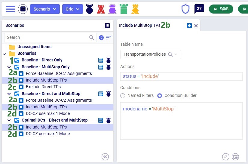
The following screenshot shows the scenarios and which scenario items are associated with each of them. To learn more about creating scenarios and their items, please see these 2 help center articles: "Creating Scenarios in Cosmic Frog" and "Getting Started with Scenarios".
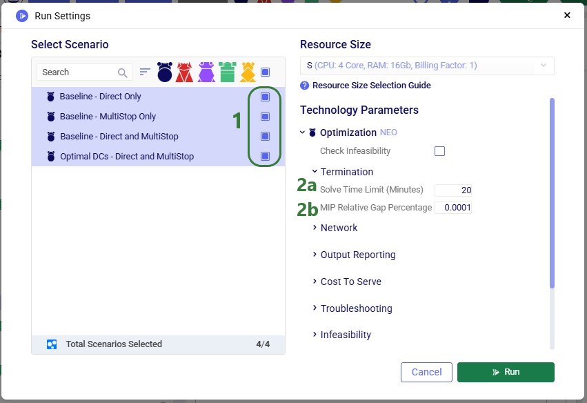
To find a balance between running the model to a low enough gap to reduce any suboptimality in the solution and running for a reasonable amount of time, the following is set on the Run Settings modal which comes up after clicking on the green Run button at the top right in Cosmic Frog:
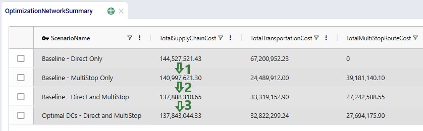
We will first look at the Optimization Network Summary and Optimization Flow Summary output tables, and next at the maps of the last 2 scenarios. We will start with the Optimization Network Summary output table. This screenshot does not show the Production and Fixed Operating Costs as they are the same across all scenarios, and we will focus on the transportation related costs:
Next, the Optimization Flow Summary output table is filtered for 1 specific customer, CZ215, for which the DC assignment is changed in the final scenario. The table is also filtered for the Rockets product, for which the delivered quantity is the same for these 4 records (1,243 units):
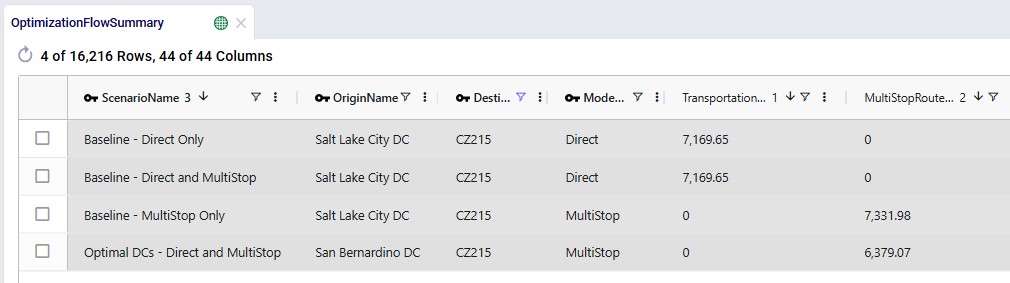
Salt Lake City is the optimal DC to source from for this customer based on just the direct delivery option; the transportation cost is ~7.2k. We see from the "Baseline - MultiStop Only" scenario that using a multi-stop route from Salt Lake City to this customer is a little more expensive (7.3k), so therefore the Direct mode is used in the "Baseline - Direct and MultiStop" scenario. In the "Optimal DCs - Direct and MultiStop" scenario, the customer swaps DC and is served using a multi-stop route from the San Bernardino DC, this results in a transportation cost of 6.4k, which is a reduction of almost $800 as compared to going direct from the Salt Lake City DC.
With a newly added output table named Optimization Flow Route Summary, we can see on which route from San Bernardino CZ215 is placed in this "Optimal" scenario:
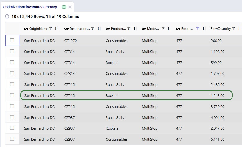
We see that CZ215 is a stop on route 477 from San Bernardino. The screenshot also shows the other stops on this route. Now we will retrace how the multi-stop route cost of $6.4k for this flow (see previous screenshot) is calculated:
When the possible routes are created during the model run, each customer is placed on up to 3 potential routes from its closest 2 DCs. These possible routes generated during preprocessing are listed in the HopperRouteSummary.csv input file which is generated when the "Write Input Solver" model run option (Troubleshooting section) is turned on. We can look up route 477 in it to see the cost for it:
The following 2 maps show the DC-CZ flows for the "Baseline - Direct and MultiStop" and "Optimal DCs - Direct and MultiStop" scenarios. Multi-stop routes are shown with blue lines and direct deliveries with red lines. There are 15 customers that swap DCs and these are shown with larger red dots:
In total 15 CZs are swapping DCs in the "Optimal DCs - Direct and MultiStop" scenario. From west to east on the map:
The last 3 swaps cause some flow lines to be crossing each other on the map. This is due to the algorithm considering a finite number of possible routes.
Note that maps for the first 2 scenarios are also set up in this demo model.
Re-running these scenarios in future with a newer solver and/or after making (small) changes to the model can change the outputs such that the set of reassigned customers which are shown in larger red dots on the map changes. To visualize these on the map in the same way as is done above, the filter in the Condition Builder panel of the "Reassigned Customers" map layer needs to be updated manually. Currently the filter is as follows:
To determine which customers are being reassigned and need to be used in this filter, users can take following steps (which can be automated using for example DataStar):
With this new functionality, a transportation optimization (Hopper) run is started immediately after a network optimization (Neo) run has completed and this will be seen as one run to the user. Underneath, the assignments on the last leg of the network (e.g. customer to DC assignments) as determined optimal by the Neo run will be fixed for the Hopper run, and then multi-stop routes are generated for this last leg during the Hopper run. All existing Hopper functionality is taken into account while determining the optimal multi-stop routes and complete sets of outputs for both the network optimization and transportation optimization are generated at the end of a Hopper after Neo run. This saves users time where they do not need to go into the model to retrieve and manipulate Neo outputs to be used as input shipments for a subsequent Hopper run.
Besides needing the usual input for the network optimization (Neo) engine to be able to run, the Hopper after Neo algorithm needs some additional inputs in order to generate optimal multi-stop routes after the Neo run has completed. These include:
In addition, all populated Hopper fields used on any other Hopper table will be used during the Hopper part of the solve.
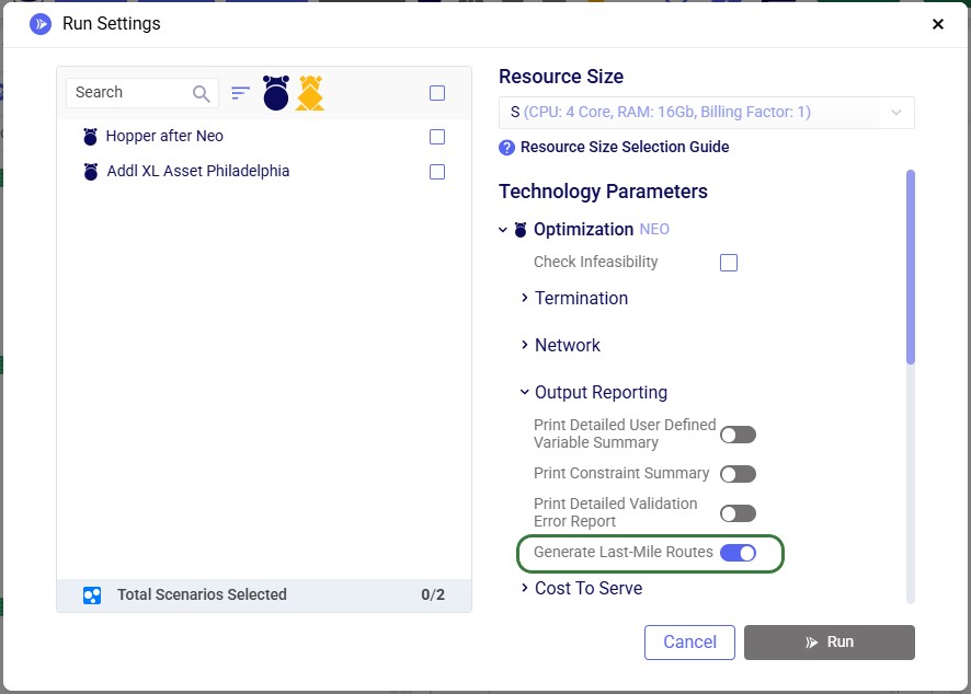
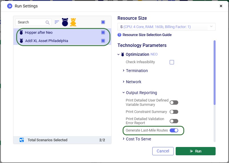
To turn on the Hopper after Neo functionality, one needs to enable the "Generate Last-Mile Routes" run setting in the Output Reporting section of the Optimization (NEO) Technology Parameters. These parameters are located on the right-hand side of the Run Settings modal which comes up after clicking on the green Run button at the right top in Cosmic Frog:
Please see the "Model used to showcase Hopper within/after Neo Features" section further above for the details of the starting point for the demo model for Hopper after Neo, which is the same one that was also the starting point for the Hopper within Neo demo model.
We will show how Hopper routes for the last leg of the network, from DCs to customers, can be created immediately after a Neo solve. Through 2 scenarios, we will explore which asset mix will be optimal for the generated multi-stop routes:
After copying the Global Supply Chain Strategy model from the Resource Library, following changes/additions were made to be able to use Hopper for multi-stop route generation for the DC-CZ leg after the Neo solve. After listing these changes here, we will explain each in more detail through screenshots further below. Users can copy this modified model with the scenarios and outputs from the Resource Library.
Instead of using the 1 large default vehicle when leaving the Transportation Assets table blank, we decide to use 2 user-defined assets initially: a large and medium one. One additional extra large asset will be added after running the first scenario with the 2 assets; it will be added to resolve unrouted shipments seen in the first scenario. The assets and their settings are shown in the following 2 screenshots:
We see that both the Medium and Large vehicle are available at all locations (Domicile Location is left blank) and their Status is set to "include", whereas the Extra Large vehicle will only be available at the Philadelphia DC in the second scenario, and its initial Status is set to "Exclude". The assets have increasing fixed costs, quantity capacities, max number of stops per route, and fixed pickup times (in minutes) by increasing asset size. The fixed delivery time is the same for all: 5 minutes per stop.
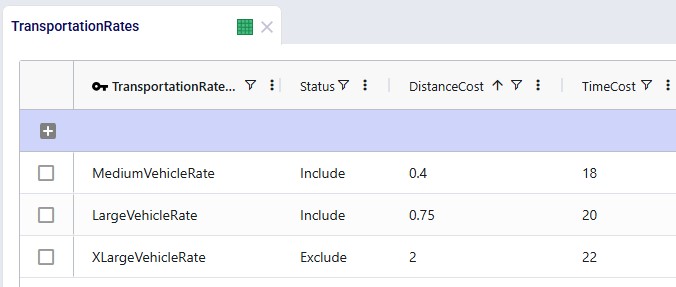
For each asset, a transportation rate is specified in the Transportation Rates input table. This rate is used in the Transportation Rate Name field in the Transportation Assets table (see screenshot above). The Distance and Time Costs are specified as follows, where the distance-based rate increases with the size of the vehicle to account for higher fuel usage. The Time Cost increases a bit with the size of the vehicle too to reflect the level of experience of the driver needed for larger vehicles:
Two scenarios will be run in this model:
When running the scenarios, the only additional input required to indicate that the Hopper engine should be run immediately after the Neo run, while taking its customer assignment decisions into account, is to turn on the "Generate Last-Mile Routes" option in the Output Reporting section of the Optimization Technology Parameters:
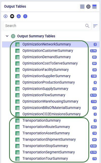
After running both scenarios, we see that full sets of outputs have been generated in the network optimization output tables and in the transportation optimization output tables:
When looking through all outputs, we notice unrouted shipments in the Transportation Shipment Summary output table. Filtering these out, we find they are all shipments coming from Philadelphia DC, and the Unrouted Reason for all = "Quantity capacity limit is reached", see the next screenshot. The large vehicle asset has a capacity of 1000 units which is not big enough to fit these shipments. Therefore, the XL asset is added at Philadelphia DC in the second scenario.
After running the second scenario, there are no more unrouted shipments and we take a look at the Transportation Summary output table which summarizes the Hopper part of the run at the scenario level. We can conclude from here that also delivering these 5 large shipments adds about $6.9k per week to the total transportation cost:
The following screenshot shows fields further to the right in the Transportation Summary output table, which confirm there are no more unrouted shipments in the second scenario, and therefore the total undelivered quantity is also 0 in this scenario:
Looking on a map, we can visualize the routes. In this example, they are colored based on which vehicle is used on the route. This is the map for the "Hopper after Neo" scenario. The map is called "Routes - Baseline" and is pre-configured when copying this model from the Resource Library:
We see that the medium asset is used for most routes from the Chicago DC and all routes from the Detroit DC; the large asset is used on all other routes.
Finally, in the next screenshot we compare the 2 scenarios side-by-side, zoomed in on the Philadelphia DC and its routes. The darker routes are those that use the XL asset. Only the 10 customers which are served by the XL asset in the second scenario are shown on the map. Six of them were served by the large asset in the "Hopper after Neo" scenario; these are shown in orange on the map. The other 4 which are colored yellow had unrouted shipments for 1 or more products in the "Hopper after Neo" scenario; three of these are clustered together northeast of Philadelphia, while one is by itself southwest of Philadelphia:
Please note that the "CZs L to XL" and "CZs Unrouted to XL" map layers contain filters on the Condition Builder pane that have been manually added after analyzing and comparing the outputs of the 2 scenarios to determine which customers to include in these layers. If the scenarios are re-run in future with a newer solver and/or after making (small) changes to the model, the outputs may change, including which customers switch from a large to extra-large vehicle and/or those going from being unrouted to using the extra-large vehicle. In that case the current condition builder filters will need to be updated to visualize those changes on the map. See the notes at the end of the "Hopper within Neo-Outputs" section which apply here in a similar way.
To determine which customers initially have unrouted shipments and are served by the extra-large vehicle in the second scenario:
To determine which customers are served by a different asset in the second scenario as compared to the first:
We hope this provides you with the guidance needed to start using the Hopper with Neo features yourself. In case of any questions, please do not hesitate to reach out to Optilogic's support team on support@optilogic.com.

Exciting new features which enable users to solve both network and transportation optimization in one solve have been added to Cosmic Frog. By optimizing multi-stop route optimization as part of Network Optimization, it enables users to streamline their analysis and make their Network Optimization more accurate. This is possible because the single optimization solve calculates multi-stop route costs by shipment/customer combination, uses this cost as part of another possible transportation mode in addition to OTR, Rail, Air, etc. and will result in more accurate answers by including better transportation costs in a single solve.
In addition to this documentation, these 2 videos cover the new Network Transportation Optimization (NTO) features too:
Network Transportation Optimization is particularly useful for two classic network design problems (both will be described in more detail in the next section):
This feature set includes 2 ways of running the Transportation Optimization (Hopper) and Network Optimization (Neo) engines together:
Following will be covered in this documentation for both the Hopper within Neo and Hopper after Neo NTO algorithms: example use cases, model inputs, how to use the new features, basics of the model used to show the NTO features, and walk through 2 example models, including their setup (input tables, scenarios), and analysis of the outputs using tables and maps.
With this feature, users can consider routes as inputs in a Neo model, meaning that the model will optimize product flow sources based on all costs, including the cost of routes. Costs and asset capacities are taken into account for the routes.
Two example use cases which can be addressed using Hopper within Neo are customer consolidation and hub optimization, which will be illustrated with the images that follow.
Consider a network where 2 distribution centers (DCs) are available to serve the customers. Two of these customers are in between the DCs and can either be serviced by the DCs directly (the blue dashed point to point lines) or product can be delivered to both of them as part of a multi-stop route from either DC (the red solid lines):
Running Neo without Hopper, not taking any route inputs into account, can lead to a solution where each DC serves 1 customer:
Whereas when taking route costs and capacities into account during a Hopper within Neo solve, it may be found that the overall cost solution is lower if one of the DCs (DC 1 in this example) serves both customers using a multi-stop route:
As a second example, consider a network where Suppliers can either deliver product to a Hub, either direct or on a multi-stop route from multiple suppliers, or direct/on multi-stop routes from multiple suppliers to a Distribution Center. Again, blue dashed lines indicate direct point to point deliveries and red lines indicate multi-stop route options:
Not taking route options into account when running Neo without Hopper can lead to a solution where each Supplier delivers to DC 1 directly:
This solution can change to one where the Suppliers deliver to the Hub on a multi-stop route when taking the route options into account in a Neo within Hopper run if this is overall beneficial (e.g. lower total cost) to do:
The Hopper within Neo algorithm needs inputs in order to consider routes as part of the Neo network optimization run. These include:
In all cases, additional records need to be added to the Transportation Policies table as well (explained in more detail below), and if the Transit Matrix table is populated, it will also be used for Hopper within Neo runs.
Please note that any other Hopper related tables (e.g. relationship constraints, business hours, transportation stop rates, etc.), whether populated or not, are not used during a Hopper within Neo solve.
To use the Hopper algorithm for route generation, the Transportation Route Planners table and Transportation Policies tables need to be used. Starting with the Transportation Route Planners table:
In the Transportation Policies table, records need to be added to indicate which lanes will be considered to be part of a multi-stop route:
Under the hood, potential routes will be calculated based on the inputs provided by the user. For example, for a case where the shipments table is not populated, and the user has specified their own assets:
As a numbers example to illustrate this calculation of a candidate route, let us consider following:
These costs are then used as inputs into the Network Optimization, together with costs for other transportation modes, and all are taken into account when optimizing the model.
To use routes that are defined by the user in the Neo solve, the user also needs to use the Transportation Route Planners table, in combination with the Fixed Routes, Fixed Routes Definitions, and Transportation Policies tables. Starting with the Transportation Route Planners table:
The Fixed Routes table connects the names of the routes the user defines with the route planner name:
There are a few additional columns on the Fixed Routes table which are not shown in the screenshot above. These are:
The Fixed Routes Definitions table needs to be used to indicate which stops are on a route together:
Please note that the Stop Number field on this table is currently not used by the Hopper within Neo functionality. The solve will determine the sequence of the stops.
Finally, to understand which locations function as sources (pickups) and which as drop-offs (deliveries) on a route, and to indicate that multi-stop routes are an option for these source-destination combinations, corresponding records need to be added to the transportation policies table too:
A copy of the Global Supply Chain Strategy model from the Resource Library was used as the starting point for both the Hopper within Neo and Hopper after Neo demo models. The original Global Supply Chain Strategy model can be found here on the Resource Library, and a video describing it can be found in this "Global Supply Chain Strategy Demo Model Review" Help Center article. The modified models showing the Hopper within and after Neo functionality can be found here on the Resource Library:
To learn more about the Resource Library and how to use it, please see the "How to use the Resource Library" Help Center article.
A short description of the main elements in this model is as follows:
We illustrate the locations and flow of product through the following 3 maps:
Even though around 35 suppliers are set up in the model in the EMEA region, only 6 of them are used based on the records in the Supplier Capabilities input table. We see the light blue lines from these suppliers delivering raw materials to the port in Rotterdam. From there, the 2 purple lines indicate the transport of the raw materials from Rotterdam to the US and Mexican ports.
Similarly, around 35 suppliers are set up in China in the model, but only 3 of them are used per the set up in the Supplier Capabilities input table. The light blue lines are the transport of raw materials from the suppliers to the Shanghai port and the purple lines from the Shanghai port to the ports in Mexico and the US.
This map shows the flows into and within/between the US and Mexico locations:
We will show how Hopper routes for the last leg of the network, from DCs to customers, can be taken into account during a Neo solve. Through a series of scenarios, we will explore if using multi-stop routes for this supply chain is beneficial:
After copying the Global Supply Chain Strategy model from the Resource Library, following changes/additions were made to be able to consider Hopper generated routes for the DC-CZ leg during the Neo solve. After listing these changes here, we will explain each in more detail through screenshots further below. Users can copy this modified model with the scenarios, outputs, and preconfigured maps from the Resource Library.
One record is added in this table where it is indicated that the route planner named "RoutePlanner_1" will use Hopper generated routes and is by default included during a Neo solve.
We choose to add our own asset instead of the 3 defaults ones that will be used if the Transportation Assets table is left blank. The characteristics of our large vehicle are shown in the next 2 screenshots:
This large asset is included in the scenario runs as its Status = Include. The fixed cost of the asset is $1,000, with a capacity of 400 units / 400 cubic feet / 400 pounds.
A rate record is set up in the Transportation Rates input table in order to model distance- and time-based costs. This is shown in the next screenshot. To use it, we link it to the asset by using the Transportation Rate Name field on the Transportation Assets table.
The Max Stops Per Route is set to 10. A Fixed Pickup Time of 15 minutes is entered, which will be applied once when picking up product at the DCs. Also, a Fixed Delivery Time of 5 minutes is set, this will be applied once at each customer when delivering product (the UOM fields are omitted in the screenshot; they are set to MIN).
Besides the fixed cost for the asset as specified in the Transportation Assets table, we also want to apply both distance- and time-based costs to the routes:
A record is set up in the Transportation Rates table where Transportation Rate Name is used in the Transportation Assets table to link the correct rate to the correct asset (e.g. LargeVehicleRate is used for the LargeVehicleAsset). The per distance cost is set to 0.9 per mile, and the time cost is set to 20 per hour; the latter mostly reflects the cost for the driver.
For the scenarios to use actual road distances and transport times, the Distance Lookup Utility in Cosmic Frog was used with following parameters:
A subset of records filtered for 1 customer destination (CZ1411) is shown in this next screenshot where we see the distance and time from the 10 closest other customers to this customer, and also from all 7 DCs:
To remove potential dual sourcing, all customers are set to single sourcing (Single Source field is set to True on the Customers table), meaning they need to be served all product they demand from a single DC. In this model, setting customers to single sourcing also helps reduce the runtime of the scenarios:
To further help reduce solve times, a flow count constraint that allows the selection of at maximum 1 mode to each customer is added:
Groups for all DCs, all Customers, all Products, and all Modes (the 2 to customers, Direct and MultiStop) are being used in the Origin, Destination, Product, and Mode fields on the Flow Count Constraints table. The Group Behavior fields for Origin and Destination are set to Enumerate, meaning that under the hood, this constraint is expanded out into individual constraints for each DC-Customer combination. On the other hand, the Group Behavior fields for Product and Mode are set to aggregate, meaning that the constraint applies to all products and modes together. The Counting Rule indicates the combination of entities that "is counted on", in this case the number of modes, which is not allowed to be more than 1 (Type = Max and Value = 1), i.e. there can only be 1 mode selected on each DC-customer lane.
The Status field of the Flow Count Constraint is set to Exclude (not shown in the screenshots above), and the constraint will be included in 2 of the scenarios by changing the status through a scenario item.
The following screenshot shows the scenarios and which scenario items are associated with each of them. To learn more about creating scenarios and their items, please see these 2 help center articles: "Creating Scenarios in Cosmic Frog" and "Getting Started with Scenarios".
To find a balance between running the model to a low enough gap to reduce any suboptimality in the solution and running for a reasonable amount of time, the following is set on the Run Settings modal which comes up after clicking on the green Run button at the top right in Cosmic Frog:
We will first look at the Optimization Network Summary and Optimization Flow Summary output tables, and next at the maps of the last 2 scenarios. We will start with the Optimization Network Summary output table. This screenshot does not show the Production and Fixed Operating Costs as they are the same across all scenarios, and we will focus on the transportation related costs:
Next, the Optimization Flow Summary output table is filtered for 1 specific customer, CZ215, for which the DC assignment is changed in the final scenario. The table is also filtered for the Rockets product, for which the delivered quantity is the same for these 4 records (1,243 units):
Salt Lake City is the optimal DC to source from for this customer based on just the direct delivery option; the transportation cost is ~7.2k. We see from the "Baseline - MultiStop Only" scenario that using a multi-stop route from Salt Lake City to this customer is a little more expensive (7.3k), so therefore the Direct mode is used in the "Baseline - Direct and MultiStop" scenario. In the "Optimal DCs - Direct and MultiStop" scenario, the customer swaps DC and is served using a multi-stop route from the San Bernardino DC, this results in a transportation cost of 6.4k, which is a reduction of almost $800 as compared to going direct from the Salt Lake City DC.
With a newly added output table named Optimization Flow Route Summary, we can see on which route from San Bernardino CZ215 is placed in this "Optimal" scenario:
We see that CZ215 is a stop on route 477 from San Bernardino. The screenshot also shows the other stops on this route. Now we will retrace how the multi-stop route cost of $6.4k for this flow (see previous screenshot) is calculated:
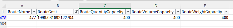
When the possible routes are created during the model run, each customer is placed on up to 3 potential routes from its closest 2 DCs. These possible routes generated during preprocessing are listed in the HopperRouteSummary.csv input file which is generated when the "Write Input Solver" model run option (Troubleshooting section) is turned on. We can look up route 477 in it to see the cost for it:
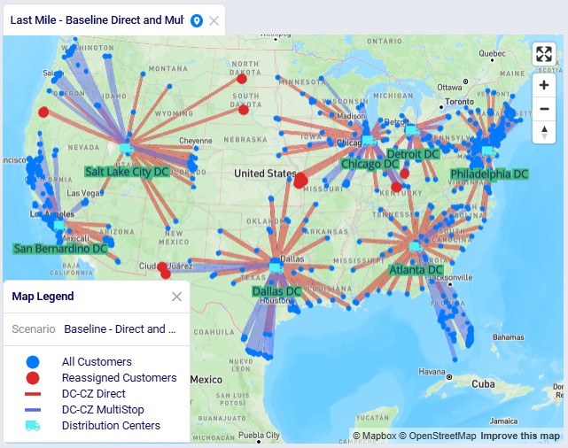
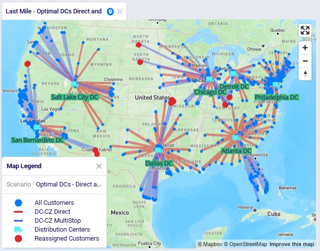
The following 2 maps show the DC-CZ flows for the "Baseline - Direct and MultiStop" and "Optimal DCs - Direct and MultiStop" scenarios. Multi-stop routes are shown with blue lines and direct deliveries with red lines. There are 15 customers that swap DCs and these are shown with larger red dots:
In total 15 CZs are swapping DCs in the "Optimal DCs - Direct and MultiStop" scenario. From west to east on the map:
The last 3 swaps cause some flow lines to be crossing each other on the map. This is due to the algorithm considering a finite number of possible routes.
Note that maps for the first 2 scenarios are also set up in this demo model.
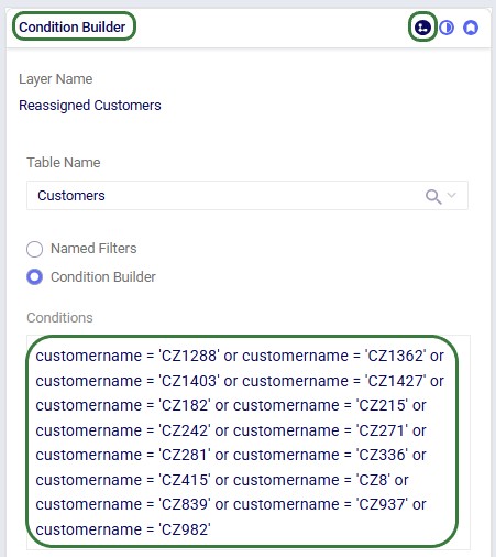
Re-running these scenarios in future with a newer solver and/or after making (small) changes to the model can change the outputs such that the set of reassigned customers which are shown in larger red dots on the map changes. To visualize these on the map in the same way as is done above, the filter in the Condition Builder panel of the "Reassigned Customers" map layer needs to be updated manually. Currently the filter is as follows:
To determine which customers are being reassigned and need to be used in this filter, users can take following steps (which can be automated using for example DataStar):
With this new functionality, a transportation optimization (Hopper) run is started immediately after a network optimization (Neo) run has completed and this will be seen as one run to the user. Underneath, the assignments on the last leg of the network (e.g. customer to DC assignments) as determined optimal by the Neo run will be fixed for the Hopper run, and then multi-stop routes are generated for this last leg during the Hopper run. All existing Hopper functionality is taken into account while determining the optimal multi-stop routes and complete sets of outputs for both the network optimization and transportation optimization are generated at the end of a Hopper after Neo run. This saves users time where they do not need to go into the model to retrieve and manipulate Neo outputs to be used as input shipments for a subsequent Hopper run.
Besides needing the usual input for the network optimization (Neo) engine to be able to run, the Hopper after Neo algorithm needs some additional inputs in order to generate optimal multi-stop routes after the Neo run has completed. These include:
In addition, all populated Hopper fields used on any other Hopper table will be used during the Hopper part of the solve.
To turn on the Hopper after Neo functionality, one needs to enable the "Generate Last-Mile Routes" run setting in the Output Reporting section of the Optimization (NEO) Technology Parameters. These parameters are located on the right-hand side of the Run Settings modal which comes up after clicking on the green Run button at the right top in Cosmic Frog:
Please see the "Model used to showcase Hopper within/after Neo Features" section further above for the details of the starting point for the demo model for Hopper after Neo, which is the same one that was also the starting point for the Hopper within Neo demo model.
We will show how Hopper routes for the last leg of the network, from DCs to customers, can be created immediately after a Neo solve. Through 2 scenarios, we will explore which asset mix will be optimal for the generated multi-stop routes:
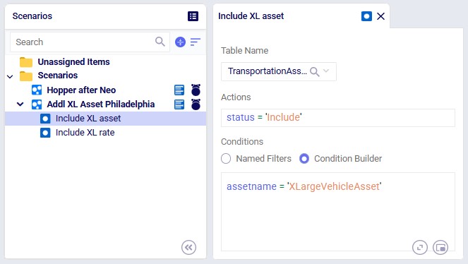
After copying the Global Supply Chain Strategy model from the Resource Library, following changes/additions were made to be able to use Hopper for multi-stop route generation for the DC-CZ leg after the Neo solve. After listing these changes here, we will explain each in more detail through screenshots further below. Users can copy this modified model with the scenarios and outputs from the Resource Library.
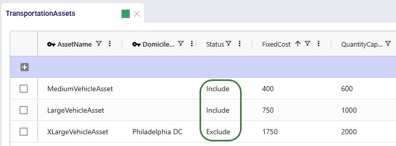
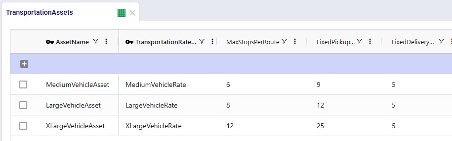
Instead of using the 1 large default vehicle when leaving the Transportation Assets table blank, we decide to use 2 user-defined assets initially: a large and medium one. One additional extra large asset will be added after running the first scenario with the 2 assets; it will be added to resolve unrouted shipments seen in the first scenario. The assets and their settings are shown in the following 2 screenshots:
We see that both the Medium and Large vehicle are available at all locations (Domicile Location is left blank) and their Status is set to "include", whereas the Extra Large vehicle will only be available at the Philadelphia DC in the second scenario, and its initial Status is set to "Exclude". The assets have increasing fixed costs, quantity capacities, max number of stops per route, and fixed pickup times (in minutes) by increasing asset size. The fixed delivery time is the same for all: 5 minutes per stop.
For each asset, a transportation rate is specified in the Transportation Rates input table. This rate is used in the Transportation Rate Name field in the Transportation Assets table (see screenshot above). The Distance and Time Costs are specified as follows, where the distance-based rate increases with the size of the vehicle to account for higher fuel usage. The Time Cost increases a bit with the size of the vehicle too to reflect the level of experience of the driver needed for larger vehicles:
Two scenarios will be run in this model:
When running the scenarios, the only additional input required to indicate that the Hopper engine should be run immediately after the Neo run, while taking its customer assignment decisions into account, is to turn on the "Generate Last-Mile Routes" option in the Output Reporting section of the Optimization Technology Parameters:
After running both scenarios, we see that full sets of outputs have been generated in the network optimization output tables and in the transportation optimization output tables:
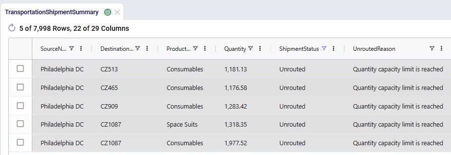
When looking through all outputs, we notice unrouted shipments in the Transportation Shipment Summary output table. Filtering these out, we find they are all shipments coming from Philadelphia DC, and the Unrouted Reason for all = "Quantity capacity limit is reached", see the next screenshot. The large vehicle asset has a capacity of 1000 units which is not big enough to fit these shipments. Therefore, the XL asset is added at Philadelphia DC in the second scenario.
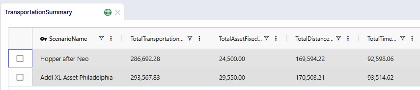
After running the second scenario, there are no more unrouted shipments and we take a look at the Transportation Summary output table which summarizes the Hopper part of the run at the scenario level. We can conclude from here that also delivering these 5 large shipments adds about $6.9k per week to the total transportation cost:
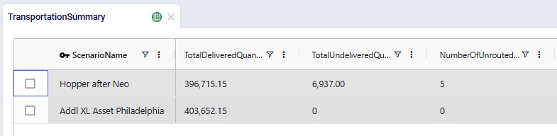
The following screenshot shows fields further to the right in the Transportation Summary output table, which confirm there are no more unrouted shipments in the second scenario, and therefore the total undelivered quantity is also 0 in this scenario:
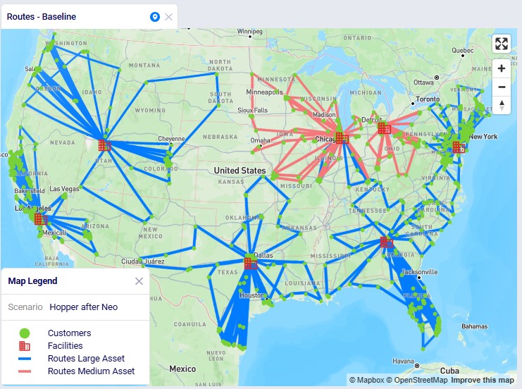
Looking on a map, we can visualize the routes. In this example, they are colored based on which vehicle is used on the route. This is the map for the "Hopper after Neo" scenario. The map is called "Routes - Baseline" and is pre-configured when copying this model from the Resource Library:
We see that the medium asset is used for most routes from the Chicago DC and all routes from the Detroit DC; the large asset is used on all other routes.
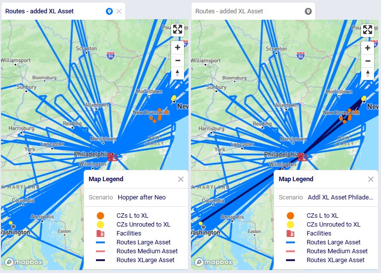
Finally, in the next screenshot we compare the 2 scenarios side-by-side, zoomed in on the Philadelphia DC and its routes. The darker routes are those that use the XL asset. Only the 10 customers which are served by the XL asset in the second scenario are shown on the map. Six of them were served by the large asset in the "Hopper after Neo" scenario; these are shown in orange on the map. The other 4 which are colored yellow had unrouted shipments for 1 or more products in the "Hopper after Neo" scenario; three of these are clustered together northeast of Philadelphia, while one is by itself southwest of Philadelphia:
Please note that the "CZs L to XL" and "CZs Unrouted to XL" map layers contain filters on the Condition Builder pane that have been manually added after analyzing and comparing the outputs of the 2 scenarios to determine which customers to include in these layers. If the scenarios are re-run in future with a newer solver and/or after making (small) changes to the model, the outputs may change, including which customers switch from a large to extra-large vehicle and/or those going from being unrouted to using the extra-large vehicle. In that case the current condition builder filters will need to be updated to visualize those changes on the map. See the notes at the end of the "Hopper within Neo-Outputs" section which apply here in a similar way.
To determine which customers initially have unrouted shipments and are served by the extra-large vehicle in the second scenario:
To determine which customers are served by a different asset in the second scenario as compared to the first:
We hope this provides you with the guidance needed to start using the Hopper with Neo features yourself. In case of any questions, please do not hesitate to reach out to Optilogic's support team on support@optilogic.com.