Territory Planning is a new capability in the Transportation Optimization (Hopper) engine that automatically clusters customers into geographic regions - territories - and restricts routes and drivers to operate within those territory boundaries. This reduces operational complexity, improves route consistency, and enables delivery-promise logic for end consumers.
Territory Planning is available today in Cosmic Frog for all users and is powered by an enhanced high-precision Genetic Algorithm. Please note that all Hopper models, whether using the new Territory Planning features or not, can now be run using this high-precision mode.
This "How-To Tutorial: Territory Planning" video explains the new feature:
In this documentation we will first cover the benefits of Territory Planning, next explain how it works in Cosmic Frog, and then take you through an example model showcasing the new feature.
Traditional routing optimization focuses on building the most cost-efficient set of routes. In many real-world operations, however, drivers do not cross territories. A driver consistently serving the same neighborhoods knows the roads, customer patterns, and service requirements.
Key benefits include:
With the Territory Planning feature one new Hopper input table and two new Hopper output tables are introduced.
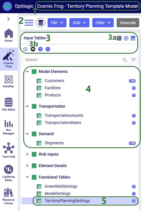
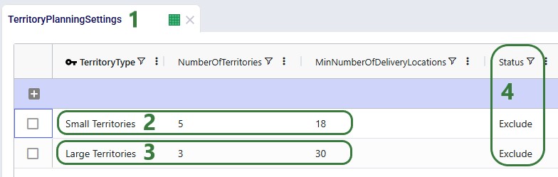
Territory Planning requires one new input table, Territory Planning Settings, while supporting all existing Hopper tables. This table defines the characteristics and constraints of the territories to be created during the Hopper solve, and can be found in the Functional Tables section: 1. Territory Type: A descriptive name for the territory configuration (e.g., "Large Territories", "Balanced Small Territories").
The universal compatibility with all other Hopper tables ensures you can add territory planning to any existing Hopper model without needing to restructure your data.
Territory Planning generates two new output tables, the Transportation Territory Planning Summary and the Transportation Territory Assignment Summary, in addition to all standard Hopper outputs. The Transportation Territory Planning Summary table provides one record per territory with aggregate KPIs:
This table is useful for:
The Transportation Territory Assignment Summary table shows the detailed assignment of each customer to a territory:
This table enables:
Besides the 2 new output tables, the following existing transportation output tables have new fields Territory Name and Territory Type added to them: Routes Map Layer, Transportation Asset Summary, Transportation Segment Summary, and Transportation Stop Summary. This facilitates filtering on territories in these tables to for example quickly see which assets are used in which territories.
Territory Planning uses Hopper's advanced genetic algorithm to simultaneously optimize multiple objectives:
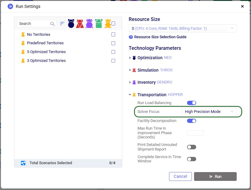
The genetic algorithm is available in Hopper's High Precision solver mode and powers all Hopper optimizations, not just territory planning. To turn on high precision mode, expand the Transportation (Hopper) section on the Run Settings modal which comes up after clicking on the green Run button at the right top in Cosmic Frog. Then select "High Precision mode" from the Solver Focus drop-down list:
A model showcasing the Territory Planning capabilities can be found here on Optilogic's Resource Library. We will cover its features, scenario configuration, and outputs here. You can copy this model to your own Optilogic account by selecting the resource and then using the Copy to Account blue button on the right hand-side (see this "How to use the Resource Library" help center article for more details).
First, we will look at the input tables of this model:
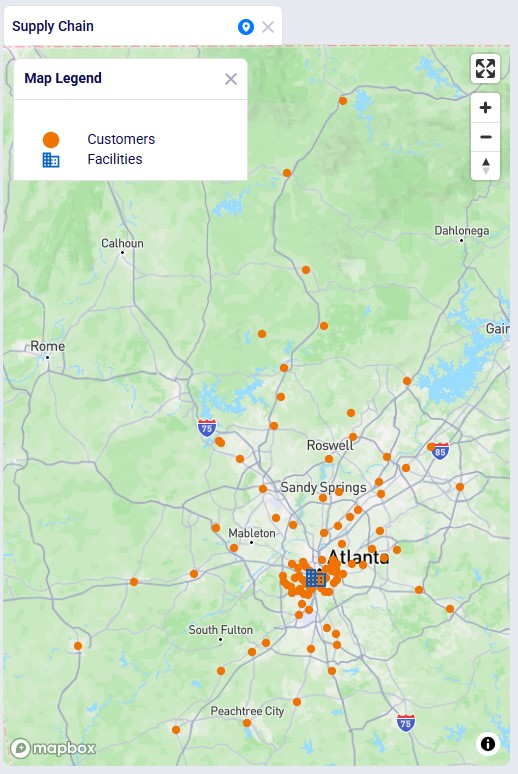
Let us also have a look at the customer and distribution center locations on the map before delving into the scenario details:
In this model, we will explore the following 4 scenarios:
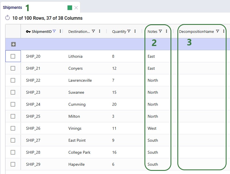
To set up the predefined territories scenario, the Notes and Decomposition Name field on the Shipments table are used:
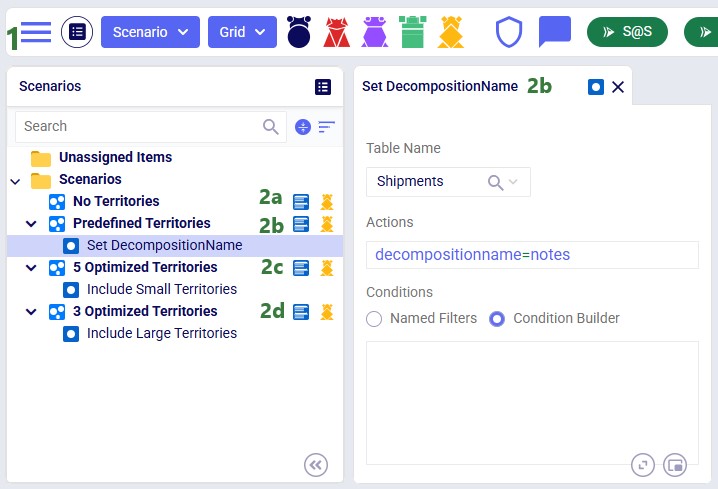
The configuration of the scenarios then looks as follows:
These scenarios are run with the Solver Focus Hopper model run option set to High Precision Mode as explained above.
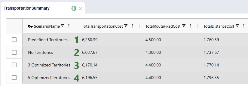
Now, we will have a look at the outputs of these 4 scenarios and compare them. First, we will look at several output tables, including the 2 new ones. We will start with the Transportation Summary output table, which summarizes costs and other KPIs at the scenario level:
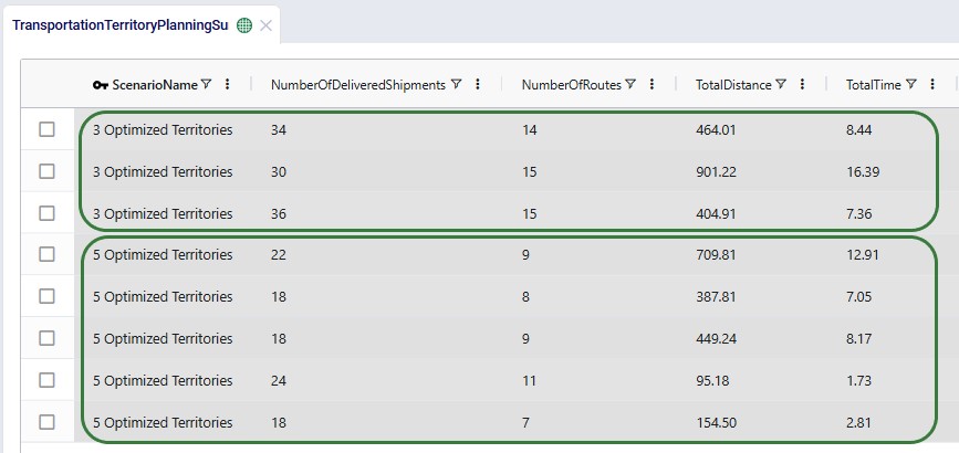
The next 2 screenshots are of the new Transportation Territory Planning Summary output table:
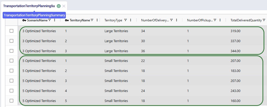
The top 3 records show the summarized outputs for each territory in the 3 Optimized Territories scenario, including the territory name and type, the number of delivery locations, the number of pickup locations, and the total delivered quantity. The bottom 5 records show the same outputs for the 5 territories of the 5 Optimized Territories scenario.
Scrolling right in this table shows additional outputs for each territory, including the number of delivered shipments, number of routes, total distance, and total time:
The other new output table, the Transportation Territory Assignment Summary table, contains the details of the assignments of customer locations to territories. The following screenshot shows the assignments of 6 customers in both the 3 Optimized Territories and 5 Optimized Territories scenarios:
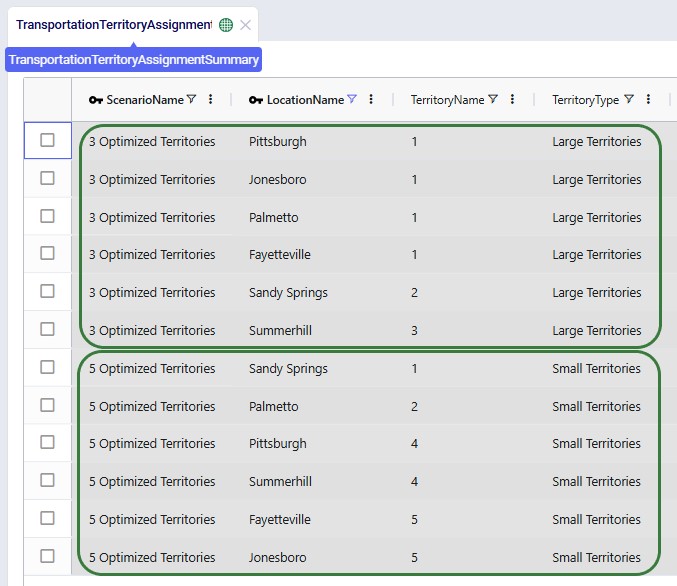
Please note that this table also includes the latitudes and longitudes of all customer locations (not shown in the screenshot), to allow easy visualization on a map.
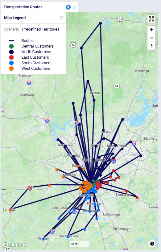
Next, we will have a look at the locations and routes on maps, these are also preconfigured in the template model that can be copied from the Resource Library, so you can have a look at these in Cosmic Frog yourself as well. The next screenshot shows the routes and locations of the Predefined Territories scenario on a map named Transportation Routes. The customers have been colored based on the predefined territory they belong to:
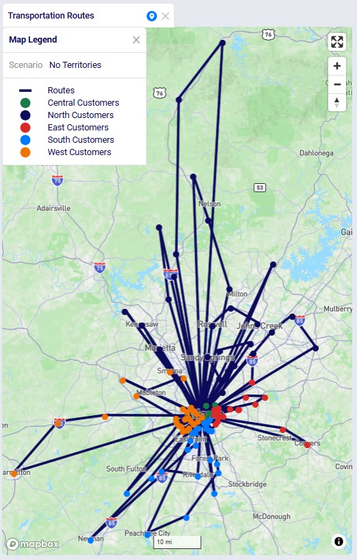
We can compare these routes to those of the No Territories scenario shown in the next screenshot. The customers are still colored based on the predefined territories, and if you zoom in a bit and pan through some routes, you will find several examples where customers from different predefined territories are now on a route together.
The following 2 screenshots compare the 3 and 5 Optimized Territories scenarios in a map called Territories Transportation Routes. The first shows the customers colored by territory. This is done by adding a layer to the map for each territory. The Transportation Stop Summary output table is used as the table to draw each of these "CZs Territory N" layers. Each layer's Condition Builder input uses "territoryname = 'N' and stoptype = 'Delivery'" as the filter; this is located on the layer's Condition Builder panel:
We see the customers clustered into their territories quite clearly in these visualizations. Some overlap between territories may happen, this can for example be due to non-uniform shipment sizes, pickup / delivery time windows, using actual road distances, etc.
This last screenshot shows the routes of the territories too, they are color coded based on the territory they belong too. This is done by again adding 1 map layer for each territory, this time drawing from the Transportation Routes Map layer table, and filtering in the Condition Builder for "territoryname = 'N'":

Territory Planning is a new capability in the Transportation Optimization (Hopper) engine that automatically clusters customers into geographic regions - territories - and restricts routes and drivers to operate within those territory boundaries. This reduces operational complexity, improves route consistency, and enables delivery-promise logic for end consumers.
Territory Planning is available today in Cosmic Frog for all users and is powered by an enhanced high-precision Genetic Algorithm. Please note that all Hopper models, whether using the new Territory Planning features or not, can now be run using this high-precision mode.
This "How-To Tutorial: Territory Planning" video explains the new feature:
In this documentation we will first cover the benefits of Territory Planning, next explain how it works in Cosmic Frog, and then take you through an example model showcasing the new feature.
Traditional routing optimization focuses on building the most cost-efficient set of routes. In many real-world operations, however, drivers do not cross territories. A driver consistently serving the same neighborhoods knows the roads, customer patterns, and service requirements.
Key benefits include:
With the Territory Planning feature one new Hopper input table and two new Hopper output tables are introduced.
Territory Planning requires one new input table, Territory Planning Settings, while supporting all existing Hopper tables. This table defines the characteristics and constraints of the territories to be created during the Hopper solve, and can be found in the Functional Tables section: 1. Territory Type: A descriptive name for the territory configuration (e.g., "Large Territories", "Balanced Small Territories").
The universal compatibility with all other Hopper tables ensures you can add territory planning to any existing Hopper model without needing to restructure your data.
Territory Planning generates two new output tables, the Transportation Territory Planning Summary and the Transportation Territory Assignment Summary, in addition to all standard Hopper outputs. The Transportation Territory Planning Summary table provides one record per territory with aggregate KPIs:
This table is useful for:
The Transportation Territory Assignment Summary table shows the detailed assignment of each customer to a territory:
This table enables:
Besides the 2 new output tables, the following existing transportation output tables have new fields Territory Name and Territory Type added to them: Routes Map Layer, Transportation Asset Summary, Transportation Segment Summary, and Transportation Stop Summary. This facilitates filtering on territories in these tables to for example quickly see which assets are used in which territories.
Territory Planning uses Hopper's advanced genetic algorithm to simultaneously optimize multiple objectives:
The genetic algorithm is available in Hopper's High Precision solver mode and powers all Hopper optimizations, not just territory planning. To turn on high precision mode, expand the Transportation (Hopper) section on the Run Settings modal which comes up after clicking on the green Run button at the right top in Cosmic Frog. Then select "High Precision mode" from the Solver Focus drop-down list:
A model showcasing the Territory Planning capabilities can be found here on Optilogic's Resource Library. We will cover its features, scenario configuration, and outputs here. You can copy this model to your own Optilogic account by selecting the resource and then using the Copy to Account blue button on the right hand-side (see this "How to use the Resource Library" help center article for more details).
First, we will look at the input tables of this model:
Let us also have a look at the customer and distribution center locations on the map before delving into the scenario details:
In this model, we will explore the following 4 scenarios:
To set up the predefined territories scenario, the Notes and Decomposition Name field on the Shipments table are used:
The configuration of the scenarios then looks as follows:
These scenarios are run with the Solver Focus Hopper model run option set to High Precision Mode as explained above.
Now, we will have a look at the outputs of these 4 scenarios and compare them. First, we will look at several output tables, including the 2 new ones. We will start with the Transportation Summary output table, which summarizes costs and other KPIs at the scenario level:
The next 2 screenshots are of the new Transportation Territory Planning Summary output table:
The top 3 records show the summarized outputs for each territory in the 3 Optimized Territories scenario, including the territory name and type, the number of delivery locations, the number of pickup locations, and the total delivered quantity. The bottom 5 records show the same outputs for the 5 territories of the 5 Optimized Territories scenario.
Scrolling right in this table shows additional outputs for each territory, including the number of delivered shipments, number of routes, total distance, and total time:
The other new output table, the Transportation Territory Assignment Summary table, contains the details of the assignments of customer locations to territories. The following screenshot shows the assignments of 6 customers in both the 3 Optimized Territories and 5 Optimized Territories scenarios:
Please note that this table also includes the latitudes and longitudes of all customer locations (not shown in the screenshot), to allow easy visualization on a map.
Next, we will have a look at the locations and routes on maps, these are also preconfigured in the template model that can be copied from the Resource Library, so you can have a look at these in Cosmic Frog yourself as well. The next screenshot shows the routes and locations of the Predefined Territories scenario on a map named Transportation Routes. The customers have been colored based on the predefined territory they belong to:
We can compare these routes to those of the No Territories scenario shown in the next screenshot. The customers are still colored based on the predefined territories, and if you zoom in a bit and pan through some routes, you will find several examples where customers from different predefined territories are now on a route together.
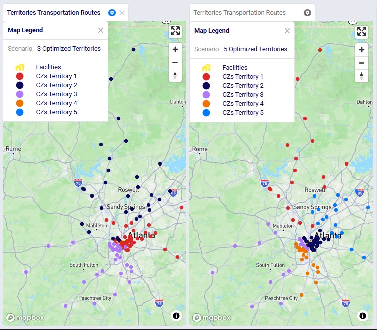
The following 2 screenshots compare the 3 and 5 Optimized Territories scenarios in a map called Territories Transportation Routes. The first shows the customers colored by territory. This is done by adding a layer to the map for each territory. The Transportation Stop Summary output table is used as the table to draw each of these "CZs Territory N" layers. Each layer's Condition Builder input uses "territoryname = 'N' and stoptype = 'Delivery'" as the filter; this is located on the layer's Condition Builder panel:
We see the customers clustered into their territories quite clearly in these visualizations. Some overlap between territories may happen, this can for example be due to non-uniform shipment sizes, pickup / delivery time windows, using actual road distances, etc.
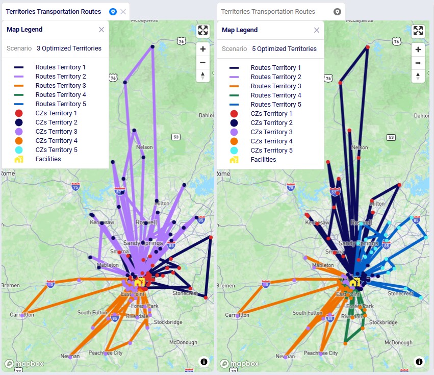
This last screenshot shows the routes of the territories too, they are color coded based on the territory they belong too. This is done by again adding 1 map layer for each territory, this time drawing from the Transportation Routes Map layer table, and filtering in the Condition Builder for "territoryname = 'N'":