When demand fluctuates due to for example seasonality, it can be beneficial to manage inventory dynamically. This means that when the demand (or forecasted demand) goes up or down, the inventory levels go up or down accordingly. To support this in Cosmic Frog models, inventory policies can be set up in terms of days of supply (DOS): for example for the (s,S) inventory policy, the Simulation Policy Value 1 UOM and Simulation Policy Value 2 UOM fields can be set to DOS. Say for example that reorder point s and order up to quantity S are set to 5 DOS and 10 DOS, respectively. This means that if the inventory falls to or below the level that is the equivalent of 5 days of supply, a replenishment order is placed that will order the amount of inventory to bring the level up to the equivalent of 10 days of supply. In this documentation we will cover the DOS-specific inputs on the Inventory Policies table, how a day of supply equivalent in units is calculated from these and walk through a numbers example.
In short, using DOS lets users be flexible with policy parameters; it is a good starting point for estimating/making assumptions about how inventory is managed in practice.
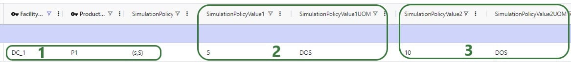
The following screenshot shows the fields that set the simulation inventory policy and its parameters:
This inventory policy for product P1 at facility DC_1 is set to (s,S) which is often referred to as a minimum/maximum policy. When the inventory falls to the value of reorder point s or below, a replenishment order is placed to bring the inventory back up to the order up to value of S.
The reorder point s is set to 5 days of supply by setting the Simulation Policy Value 1 field to 5 and its UOM field to DOS.
The order up to quantity S is set to 10 days of supply by setting the Simulation Policy Value 2 field to 10 and its UOM field to DOS.
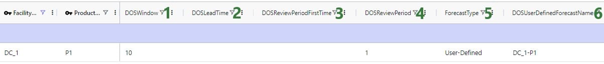
For the same inventory policy, the next screenshot shows the DOS-related fields on the Inventory Policies table; note that the UOM fields are omitted in this screenshot:
DOS Window and its UOM field – the number of days of (forecasted) demand that are used to calculate the 1 day of supply equivalent in units. Note that the default for the UOM field is hours, so it needs to be set to DAY if wanting to fill out a number in the DOS Window field that means days. In this example, the DOS Window is set to 10 days (the UOM field that is not shown is set to DAY). In practice, a DOS Window needs to be short enough to capture changes in order trends, but also long enough so that replenishments can keep up with customer orders.
DOS Leadtime and its UOM field – when using forecasted demand to calculate the 1 DOS equivalent, a lead-time can be set using these fields, so that the calculation of 1 DOS will not use the forecasted demand for the current day and immediately following days but is offset by this lead-time. This can account for the time it takes to get a replenishment order in, so the amount to reorder depends on future demand that will occur from when the replenishment arrives. Like for the DOS Window, note that the default for the UOM field is hours, so it needs to be set to DAY if wanting to fill out a number in the DOS Leadtime field that means days. Leaving this field blank is equivalent to setting it to 0, e.g. no lead-time is used for the DOS calculations.
DOS Review Period First Time – the first time during the simulation that the 1 DOS equivalent is being calculated. When left blank this is at the start of the simulation.
DOS Review Period and its UOM field – the time in between calculations of the 1 DOS equivalent. If set to 7 DAY for example, then the 1 DOS value is calculated once a week and it then stays at that value until the next DOS calculation 1 week later. Again, note that the default for the UOM field is hours, so it needs to be set to DAY if wanting to fill out a number in the DOS Review Period field that means days.
Forecast Type – this field specifies if the DOS calculations should use historical demand or forecasted demand. When set to Historical, the orders in the Customer Orders / Customer Order Profiles tables are used for the DOS calculations. When set to User-Defined, the forecasted demand that is set up using the User Defined Forecasts Data and User Defined Forecasts tables is used for the DOS calculations. Users can learn more about the Customer Orders / Customer Order Profiles tables in this help center article called “Adding Demand (Simulation)”. The User Defined Forecasts Data and User Defined Forecasts tables are covered below in the next section.
Note that an important difference between using historical vs forecasted demand is that Customer Orders / Customer Order Profiles are entered at the customer-product level, whereas forecasted demand needs to be specified at the facility-product level. For historical demand specified in the Customer Orders / Customer Order Profiles tables, the demand to multiple customers that is filled by 1 facility will be automatically aggregated by Cosmic Frog for the purpose of inventory management.
DOS User Defined Forecast Name – when Forecast Type is set to User-Defined, this field specifies the name of the forecast (set up in the User Defined Forecasts Data and User Defined Forecasts tables, covered below) to be used for the DOS calculations.
User-Defined Forecasts
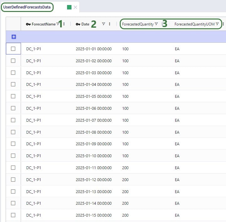
As mentioned above, when using forecasted demand for the DOS calculations, this forecasted demand needs to be specified in the User Defined Forecasts Data and User Defined Forecasts tables, which we will discuss here. This next screenshot shows the first 15 example records in the User Defined Forecasts Table:
Forecast Name – the name of the forecast being specified. Records with the same Forecast Name together make up a forecast.
Date – date and optionally time at which the forecasted demand occurs.
Forecasted Quantity and its UOM field – the amount of product that is forecasted to be demanded on the specified date.
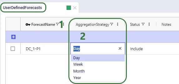
Next, the User Defined Forecasts table lets a user configure the time-period to which a forecast is aggregated:
Forecast Name – this should match the name of a forecast specified in the User Defined Forecasts Data table.
Aggregation Strategy – select if a forecast should be rolled up to the day, week, month or year level.
DOS Calculations
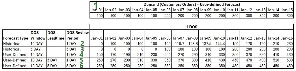
Let us now explain how the DOS calculations work for different DOS settings through the examples shown in the next screenshot. Note that for all these examples the DOS Review Period First Time field has been left blank, meaning that the first 1 DOS equivalent calculation occurs at the start of this model (on January 1st) for each of these examples:
For convenience’s sake, we are assuming that the historical demand (specified in the Customer Orders /Customer Order Profiles tables) rolled up to the facility-product combination is the same as the forecasted demand at this facility-product combination as set up in the User Defined Forecasts Data table. For January 1st through January 5th, the (forecasted) demand for DC_1 – P1 is 100 units, for January 6th-10th it is 200 units, for January 11th-15th it is 300 units. This pattern of increasing by 100 every 5 days continues in the future although not shown in the table above: 400 units for January 16th-20th, 500 units for January 21st-25th, etc.
When using historical demand with a 10 day DOS Window and 1 day DOS Review Period, the calculation of 1 DOS on January 1st uses the historical demand occurring during the 10 days before January 1st: December 22nd through December 31st of the previous year. However, this model starts on January 1st and there is no customer order data for these 10 days in December in the model. Therefore, the calculation of 1 DOS results in 0. Since DOS Review Period is set to 1 day, the next time the 1 DOS equivalent is calculated is on January 2nd: there is now 1 day of history that the model will use for the calculation: the demand on January 1st is 100, so the equivalent of 1 DOS on January 2nd = 100 (sum daily demand Jan 1) / 1 (day) = 100. For the next DOS review on January 3rd, there are 2 historical demand records available to use and the 1 DOS calculation is as follows: 200 (sum of daily demand Jan 1-2) / 2 (days) = 100. Since the demand does not change for several days, the average daily demand (or 1 DOS) does not change until the demand goes up to 200 on January 6th. The 1 DOS calculation for January 7th becomes: 700 (sum of daily demand Jan 1-6) / 6 (days) = 116.7. On January 11th there is finally enough historical demand to use the full 10 days of the DOS window and the 1 DOS equivalent calculation becomes: 1,500 (sum daily demand Jan 1-10) / 10 (days) = 150. The calculation on Jan 12th uses the demand for Jan 2-11: 1,700 (sum daily demand Jan 2-11) / 10 (days) = 170, etc.
The next record shows the results of the 1 DOS calculation when again using historical demand, but now with a 5 day DOS Window and a 5 day DOS Review Period. For the 1 DOS equivalent calculation for January 1st there is again no history in the model, so it results in 0. But now, since the DOS Review Period is set to 5 days, the next DOS review is on January 6th and the 1 DOS equivalent of 0 as calculated on January 1st will be used until then as the 1 DOS equivalent. On January 6th, the 1 DOS calculation is as follows: 500 (sum of daily demand Jan 1-5) / 5 (days) = 100. Again, it stays at this value of 100 throughout January 10th, since the next review is on January 11th. On this day, January 11, we use the demand for January 6-10 to calculate 1 DOS since the DOS Window is set to 5 days, so the result is: 1,000 (sum daily demand Jan 6-10) / 5 (days) = 200, etc.
This example and the next 2 use forecasted demand since the Forecast Type is set to User-Defined. For this record, the DOS Window is set to 10 days, there is no DOS Lead-time and the DOS Review Period is 1 day. For the DOS calculation on January 1st, the model looks forward at the forecasted demand for the next 10 days starting on January 1: 1,500 (sum of daily demand Jan 1-10) / 10 (days) = 150. With a DOS Review Period of 1 day, the next 1 DOS equivalent calculation is on January 2nd: 1,700 (sum daily demand Jan 2-11) / 10 (days) = 170, etc.
This next example also uses forecasted demand, a 10 day DOS Window, and 1 day DOS Review Period like the previous example discussed under bullet 4. The only difference is that in this example there is also a 5 day DOS Lead-time specified. This means that on January 1 we do not use the forecasted demand for Jan 1-10, but we offset it by 5 days to start on January 6. The 1 DOS equivalent calculated on January 1 is therefore: 2,500 (sum daily demand Jan 6-15) / 10 (days) = 250. Since DOS Review Period is 1 day, the next 1 DOS equivalent calculation is on January 2nd and is as follows: 2,700 (sum daily demand Jan 7-16) / 10 (days) = 270, etc.
Our last example is the same as the previous one under bullet 5 with the 1 change that the DOS Review Period is changed to 5 days (from 1 day). The 1 DOS calculation on January 1st is the same as for the previous bullet and results in 250. The 1 DOS equivalent stays at 250 until the next DOS review occurs on January 6th, which uses the forecasted demand for January 11-20 and the 1 DOS equivalent calculation results in: 3,500 (sum daily demand Jan 11-20) / 10 (days) = 350. It again stays at this value for 5 days until the next DOS review on January 11th, etc.
Inventory Policy using DOS – Numbers Example
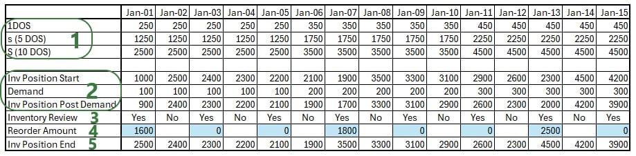
Now that we know how to calculate the value of 1 DOS, we can apply this to inventory policies which use DOS as their UOM for the simulation policy value fields. We will do a numbers example with the one shown in the screenshot above (in the Days of Supply Settings section) where reorder point s is 5 DOS and order up to quantity S is 10 DOS. Let us assume the same settings as in the last example for the 1 DOS calculations in the screenshot above, explained in bullet #6 above: forecasted demand is used with a 10 day DOS Window, a 5 day DOS Leadtime, and a 5 day DOS Review Period, so the calculations for the equivalent of 1 DOS are the numbers in the last row shown in the screenshot, which we will use in our example below. In addition to this, we will assume a 2 day Review Period for the inventory policy, meaning inventory levels are checked every other day to see if a replenishment order needs to be placed. DC_1 also has 1,000 units of P1 on hand at the start of the simulation (specified in the Initial Inventory field):
The first record shows the same numbers for the equivalent of 1 DOS for January 1-15 as calculated in the last record of the previous screenshot and explained under bullet #6 above. From this 1 DOS equivalent, we calculate the reorder point, which is 5 DOS, and the order up to quantity, which is 10 DOS for each day in the January 1-15 period.
The next 3 rows show the starting inventory position on the day, the forecasted demand for that day, and the inventory position after the forecasted demand is subtracted from the starting inventory.
The inventory review record indicates if inventory is reviewed on that day. As mentioned, the Review Period is set to 2 days, so inventory is reviewed every other. The first review is at the start of the simulation on January 1st, the next on January 3rd, then January 5th, etc.
On the days where inventory is reviewed, it is determined if a replenishment order needs to be placed, and if so, for how many units. To do so, the Inventory Position Post Demand is compared with the reorder point s and if it is at the value of the reorder point or below, a replenishment order will be placed. If an order is placed, the amount will be so that the inventory position is brought back up to the value of the order up to quantity S. On January 1st, the reorder point s is 1,250 and the inventory position post demand is 900. Therefore, a replenishment order will be placed as the inventory position is below the reorder point (900 < 1,250). The order up to quantity S is 2,500 on January 1st, so 2,500 (order up to) – 900 (inv position post demand) = 1,600 units will be ordered. On January 3rd and 5th, the inventory positions after filling demand are greater than the reorder point (2,300 > 1,250 and 2,100 > 1,250, respectively). At the next review on January 7th, a replenishment order is placed as the inventory position post demand (1,700) is less than the reorder point (1,750). The amount to reorder is calculated to be 3,500 (order up to quantity S) – 1,700 (inventory position post demand) = 1,800, etc.
The inventory position end indicates the inventory position at the end of the day and is used as the starting inventory position for the next day.
When demand fluctuates due to for example seasonality, it can be beneficial to manage inventory dynamically. This means that when the demand (or forecasted demand) goes up or down, the inventory levels go up or down accordingly. To support this in Cosmic Frog models, inventory policies can be set up in terms of days of supply (DOS): for example for the (s,S) inventory policy, the Simulation Policy Value 1 UOM and Simulation Policy Value 2 UOM fields can be set to DOS. Say for example that reorder point s and order up to quantity S are set to 5 DOS and 10 DOS, respectively. This means that if the inventory falls to or below the level that is the equivalent of 5 days of supply, a replenishment order is placed that will order the amount of inventory to bring the level up to the equivalent of 10 days of supply. In this documentation we will cover the DOS-specific inputs on the Inventory Policies table, how a day of supply equivalent in units is calculated from these and walk through a numbers example.
In short, using DOS lets users be flexible with policy parameters; it is a good starting point for estimating/making assumptions about how inventory is managed in practice.
The following screenshot shows the fields that set the simulation inventory policy and its parameters:
This inventory policy for product P1 at facility DC_1 is set to (s,S) which is often referred to as a minimum/maximum policy. When the inventory falls to the value of reorder point s or below, a replenishment order is placed to bring the inventory back up to the order up to value of S.
The reorder point s is set to 5 days of supply by setting the Simulation Policy Value 1 field to 5 and its UOM field to DOS.
The order up to quantity S is set to 10 days of supply by setting the Simulation Policy Value 2 field to 10 and its UOM field to DOS.
For the same inventory policy, the next screenshot shows the DOS-related fields on the Inventory Policies table; note that the UOM fields are omitted in this screenshot:
DOS Window and its UOM field – the number of days of (forecasted) demand that are used to calculate the 1 day of supply equivalent in units. Note that the default for the UOM field is hours, so it needs to be set to DAY if wanting to fill out a number in the DOS Window field that means days. In this example, the DOS Window is set to 10 days (the UOM field that is not shown is set to DAY). In practice, a DOS Window needs to be short enough to capture changes in order trends, but also long enough so that replenishments can keep up with customer orders.
DOS Leadtime and its UOM field – when using forecasted demand to calculate the 1 DOS equivalent, a lead-time can be set using these fields, so that the calculation of 1 DOS will not use the forecasted demand for the current day and immediately following days but is offset by this lead-time. This can account for the time it takes to get a replenishment order in, so the amount to reorder depends on future demand that will occur from when the replenishment arrives. Like for the DOS Window, note that the default for the UOM field is hours, so it needs to be set to DAY if wanting to fill out a number in the DOS Leadtime field that means days. Leaving this field blank is equivalent to setting it to 0, e.g. no lead-time is used for the DOS calculations.
DOS Review Period First Time – the first time during the simulation that the 1 DOS equivalent is being calculated. When left blank this is at the start of the simulation.
DOS Review Period and its UOM field – the time in between calculations of the 1 DOS equivalent. If set to 7 DAY for example, then the 1 DOS value is calculated once a week and it then stays at that value until the next DOS calculation 1 week later. Again, note that the default for the UOM field is hours, so it needs to be set to DAY if wanting to fill out a number in the DOS Review Period field that means days.
Forecast Type – this field specifies if the DOS calculations should use historical demand or forecasted demand. When set to Historical, the orders in the Customer Orders / Customer Order Profiles tables are used for the DOS calculations. When set to User-Defined, the forecasted demand that is set up using the User Defined Forecasts Data and User Defined Forecasts tables is used for the DOS calculations. Users can learn more about the Customer Orders / Customer Order Profiles tables in this help center article called “Adding Demand (Simulation)”. The User Defined Forecasts Data and User Defined Forecasts tables are covered below in the next section.
Note that an important difference between using historical vs forecasted demand is that Customer Orders / Customer Order Profiles are entered at the customer-product level, whereas forecasted demand needs to be specified at the facility-product level. For historical demand specified in the Customer Orders / Customer Order Profiles tables, the demand to multiple customers that is filled by 1 facility will be automatically aggregated by Cosmic Frog for the purpose of inventory management.
DOS User Defined Forecast Name – when Forecast Type is set to User-Defined, this field specifies the name of the forecast (set up in the User Defined Forecasts Data and User Defined Forecasts tables, covered below) to be used for the DOS calculations.
User-Defined Forecasts
As mentioned above, when using forecasted demand for the DOS calculations, this forecasted demand needs to be specified in the User Defined Forecasts Data and User Defined Forecasts tables, which we will discuss here. This next screenshot shows the first 15 example records in the User Defined Forecasts Table:
Forecast Name – the name of the forecast being specified. Records with the same Forecast Name together make up a forecast.
Date – date and optionally time at which the forecasted demand occurs.
Forecasted Quantity and its UOM field – the amount of product that is forecasted to be demanded on the specified date.
Next, the User Defined Forecasts table lets a user configure the time-period to which a forecast is aggregated:
Forecast Name – this should match the name of a forecast specified in the User Defined Forecasts Data table.
Aggregation Strategy – select if a forecast should be rolled up to the day, week, month or year level.
DOS Calculations
Let us now explain how the DOS calculations work for different DOS settings through the examples shown in the next screenshot. Note that for all these examples the DOS Review Period First Time field has been left blank, meaning that the first 1 DOS equivalent calculation occurs at the start of this model (on January 1st) for each of these examples:
For convenience’s sake, we are assuming that the historical demand (specified in the Customer Orders /Customer Order Profiles tables) rolled up to the facility-product combination is the same as the forecasted demand at this facility-product combination as set up in the User Defined Forecasts Data table. For January 1st through January 5th, the (forecasted) demand for DC_1 – P1 is 100 units, for January 6th-10th it is 200 units, for January 11th-15th it is 300 units. This pattern of increasing by 100 every 5 days continues in the future although not shown in the table above: 400 units for January 16th-20th, 500 units for January 21st-25th, etc.
When using historical demand with a 10 day DOS Window and 1 day DOS Review Period, the calculation of 1 DOS on January 1st uses the historical demand occurring during the 10 days before January 1st: December 22nd through December 31st of the previous year. However, this model starts on January 1st and there is no customer order data for these 10 days in December in the model. Therefore, the calculation of 1 DOS results in 0. Since DOS Review Period is set to 1 day, the next time the 1 DOS equivalent is calculated is on January 2nd: there is now 1 day of history that the model will use for the calculation: the demand on January 1st is 100, so the equivalent of 1 DOS on January 2nd = 100 (sum daily demand Jan 1) / 1 (day) = 100. For the next DOS review on January 3rd, there are 2 historical demand records available to use and the 1 DOS calculation is as follows: 200 (sum of daily demand Jan 1-2) / 2 (days) = 100. Since the demand does not change for several days, the average daily demand (or 1 DOS) does not change until the demand goes up to 200 on January 6th. The 1 DOS calculation for January 7th becomes: 700 (sum of daily demand Jan 1-6) / 6 (days) = 116.7. On January 11th there is finally enough historical demand to use the full 10 days of the DOS window and the 1 DOS equivalent calculation becomes: 1,500 (sum daily demand Jan 1-10) / 10 (days) = 150. The calculation on Jan 12th uses the demand for Jan 2-11: 1,700 (sum daily demand Jan 2-11) / 10 (days) = 170, etc.
The next record shows the results of the 1 DOS calculation when again using historical demand, but now with a 5 day DOS Window and a 5 day DOS Review Period. For the 1 DOS equivalent calculation for January 1st there is again no history in the model, so it results in 0. But now, since the DOS Review Period is set to 5 days, the next DOS review is on January 6th and the 1 DOS equivalent of 0 as calculated on January 1st will be used until then as the 1 DOS equivalent. On January 6th, the 1 DOS calculation is as follows: 500 (sum of daily demand Jan 1-5) / 5 (days) = 100. Again, it stays at this value of 100 throughout January 10th, since the next review is on January 11th. On this day, January 11, we use the demand for January 6-10 to calculate 1 DOS since the DOS Window is set to 5 days, so the result is: 1,000 (sum daily demand Jan 6-10) / 5 (days) = 200, etc.
This example and the next 2 use forecasted demand since the Forecast Type is set to User-Defined. For this record, the DOS Window is set to 10 days, there is no DOS Lead-time and the DOS Review Period is 1 day. For the DOS calculation on January 1st, the model looks forward at the forecasted demand for the next 10 days starting on January 1: 1,500 (sum of daily demand Jan 1-10) / 10 (days) = 150. With a DOS Review Period of 1 day, the next 1 DOS equivalent calculation is on January 2nd: 1,700 (sum daily demand Jan 2-11) / 10 (days) = 170, etc.
This next example also uses forecasted demand, a 10 day DOS Window, and 1 day DOS Review Period like the previous example discussed under bullet 4. The only difference is that in this example there is also a 5 day DOS Lead-time specified. This means that on January 1 we do not use the forecasted demand for Jan 1-10, but we offset it by 5 days to start on January 6. The 1 DOS equivalent calculated on January 1 is therefore: 2,500 (sum daily demand Jan 6-15) / 10 (days) = 250. Since DOS Review Period is 1 day, the next 1 DOS equivalent calculation is on January 2nd and is as follows: 2,700 (sum daily demand Jan 7-16) / 10 (days) = 270, etc.
Our last example is the same as the previous one under bullet 5 with the 1 change that the DOS Review Period is changed to 5 days (from 1 day). The 1 DOS calculation on January 1st is the same as for the previous bullet and results in 250. The 1 DOS equivalent stays at 250 until the next DOS review occurs on January 6th, which uses the forecasted demand for January 11-20 and the 1 DOS equivalent calculation results in: 3,500 (sum daily demand Jan 11-20) / 10 (days) = 350. It again stays at this value for 5 days until the next DOS review on January 11th, etc.
Inventory Policy using DOS – Numbers Example
Now that we know how to calculate the value of 1 DOS, we can apply this to inventory policies which use DOS as their UOM for the simulation policy value fields. We will do a numbers example with the one shown in the screenshot above (in the Days of Supply Settings section) where reorder point s is 5 DOS and order up to quantity S is 10 DOS. Let us assume the same settings as in the last example for the 1 DOS calculations in the screenshot above, explained in bullet #6 above: forecasted demand is used with a 10 day DOS Window, a 5 day DOS Leadtime, and a 5 day DOS Review Period, so the calculations for the equivalent of 1 DOS are the numbers in the last row shown in the screenshot, which we will use in our example below. In addition to this, we will assume a 2 day Review Period for the inventory policy, meaning inventory levels are checked every other day to see if a replenishment order needs to be placed. DC_1 also has 1,000 units of P1 on hand at the start of the simulation (specified in the Initial Inventory field):
The first record shows the same numbers for the equivalent of 1 DOS for January 1-15 as calculated in the last record of the previous screenshot and explained under bullet #6 above. From this 1 DOS equivalent, we calculate the reorder point, which is 5 DOS, and the order up to quantity, which is 10 DOS for each day in the January 1-15 period.
The next 3 rows show the starting inventory position on the day, the forecasted demand for that day, and the inventory position after the forecasted demand is subtracted from the starting inventory.
The inventory review record indicates if inventory is reviewed on that day. As mentioned, the Review Period is set to 2 days, so inventory is reviewed every other. The first review is at the start of the simulation on January 1st, the next on January 3rd, then January 5th, etc.
On the days where inventory is reviewed, it is determined if a replenishment order needs to be placed, and if so, for how many units. To do so, the Inventory Position Post Demand is compared with the reorder point s and if it is at the value of the reorder point or below, a replenishment order will be placed. If an order is placed, the amount will be so that the inventory position is brought back up to the value of the order up to quantity S. On January 1st, the reorder point s is 1,250 and the inventory position post demand is 900. Therefore, a replenishment order will be placed as the inventory position is below the reorder point (900 < 1,250). The order up to quantity S is 2,500 on January 1st, so 2,500 (order up to) – 900 (inv position post demand) = 1,600 units will be ordered. On January 3rd and 5th, the inventory positions after filling demand are greater than the reorder point (2,300 > 1,250 and 2,100 > 1,250, respectively). At the next review on January 7th, a replenishment order is placed as the inventory position post demand (1,700) is less than the reorder point (1,750). The amount to reorder is calculated to be 3,500 (order up to quantity S) – 1,700 (inventory position post demand) = 1,800, etc.
The inventory position end indicates the inventory position at the end of the day and is used as the starting inventory position for the next day.