Cosmic Frog’s network optimization engine (Neo) can now account for shelf life and maturation time of products out of the box with the addition of several fields to the Products input table. The age of product that is used in production, product which flows between locations, and product sitting in inventory is now also reported in 3 new output tables, so users have 100% visibility into the age of their products across the operations.
In this documentation, we will give a brief overview of the new features first and then walk through a small demo model, which users can copy from the Resource Library, showing both shelf life and maturation time using 3 scenarios.
The new feature set consists of:
Please note that:
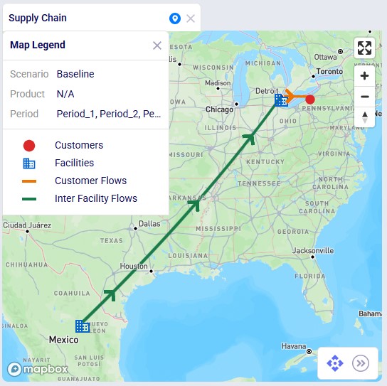
We will now showcase the use of both Shelf Life and Maturation Time in a small demo model. This model can be copied to your own Optilogic account from the Resource Library (see also the “How to use the Resource Library” Help Center article). This model has 3 locations which are shown on the map below:
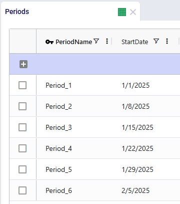
It is a multi-period model with 6 periods, which are each 1 week long (the Model End Date is set to February 12, 2025, on the Model Settings input table, not shown):
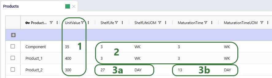
There are 3 products included the model: 2 finished goods, Product_1 and Product_2, and 1 raw material, named Component. The component is used in a bill of materials to produce Product_1, as we will see in the screenshots after this one.
As mentioned above, a bill of materials is used to produce finished good Product_1:
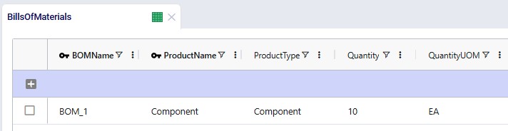
This bill of materials is named BOM_1 and it specifies that 10 units of the product named Component are used as an input (product type = Component) of this bill of materials. Note that the bill of materials does not indicate the end product that is produced with it. This is specified by associating production policies with a BOM. To learn more about detailed production modelling using the Neo engine, please see this Help Center article.
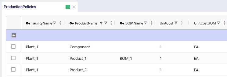
In the next screenshot of the production policies table, we see that the plant can produce all 3 products, and that for the production of Product_1, the bill of materials shown in the previous screenshot, BOM_1, is used. The cost per unit is set to 1 here for each product:
For purposes of showing how Shelf Life and Maturation Time work, we will use the Production Policies Multi-Time Period input table too. In here we override the production cost per unit that we just saw in the above screenshot to become increasingly expensive in later periods for all products, adding $1 per unit for each next period. So, to produce a unit of Product_1 in Period_1 costs $1, in Period_2 it costs $2, in Period_3 $3, etc. Same for Component and Product_2:
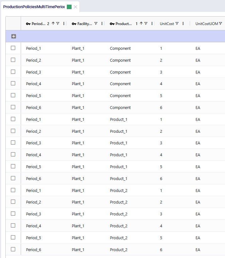
The production cost is increased here to encourage the model to produce product as early as possible, so that it incurs the lowest possible production cost. It will also still need to respect the shelf life and maturation time requirements. Note that this is also weighed against the increased inventory holding costs for producing earlier than possibly needed, as product will sit in inventory longer if produced earlier. So, the cost differential for production in different periods needs to be sufficiently big as compared to the increased inventory holding cost to see this behavior. We will explore this more through the scenarios that are run in this demo model.
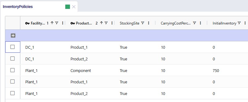
Since products will be spending some time in inventory, we need to have at least 1 inventory policy per product with Stocking Site = True. At the plant, all 3 products can be held in inventory, and there is an initial inventory of 750 units of the Component. At the DC, both finished goods can be held in inventory. The carrying cost percentage to calculate the inventory holding costs is set to 10% for all policies:
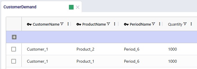
Lastly, we will show the demand that has been entered into the Customer Demand table. The customer demands 1,000 units each of the finished goods in period #6:
Other input tables that have populated records which have not been shown in a screenshot above are: Customers, Facilities, and Transportation Policies. The latter specifies that the plant can ship both finished goods to the DC, and the DC can ship both to the customer. The cost of transportation is set to 0.01 per unit per mile on both lanes.
The 3 costs that are modelled are therefore:
There are 3 scenarios run in this model, see also the screenshot below:
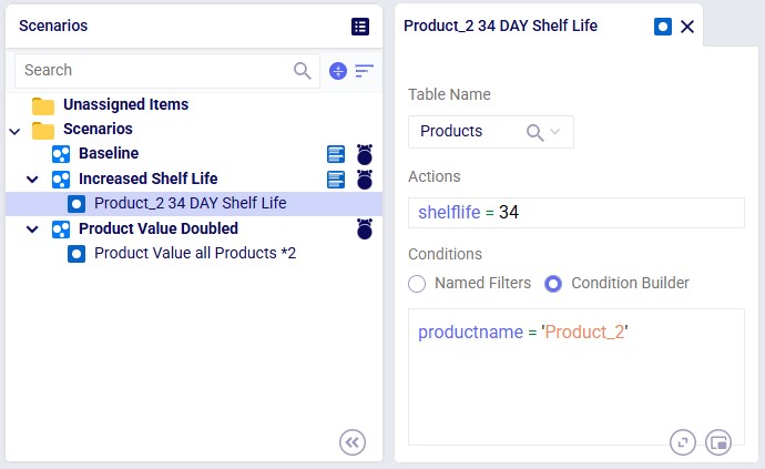
The screenshot shows the 3 scenarios on the left, where we see that the Increased Shelf Life and Product Value Doubled scenarios both contain 1 scenario item, whereas the Baseline does not contain any. On the right-hand side, the scenario item of the Increased Shelf Life scenario is shown where we can see that the Shelf Life value of Product_2 is set to 34. See the following Help Center articles for more details on Scenario building and syntax:
Two notes upfront about the outputs before we dive into details as follows:
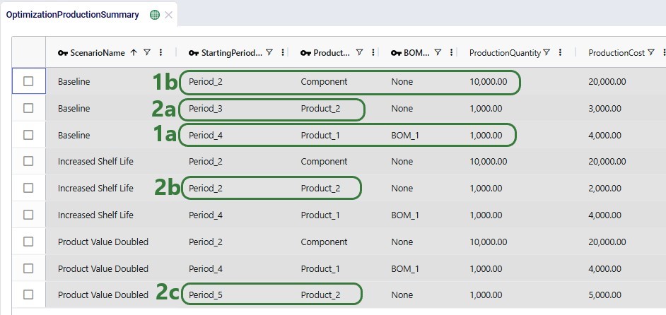
Now let us first look at when which product is produced through the Optimization Production Summary output table:
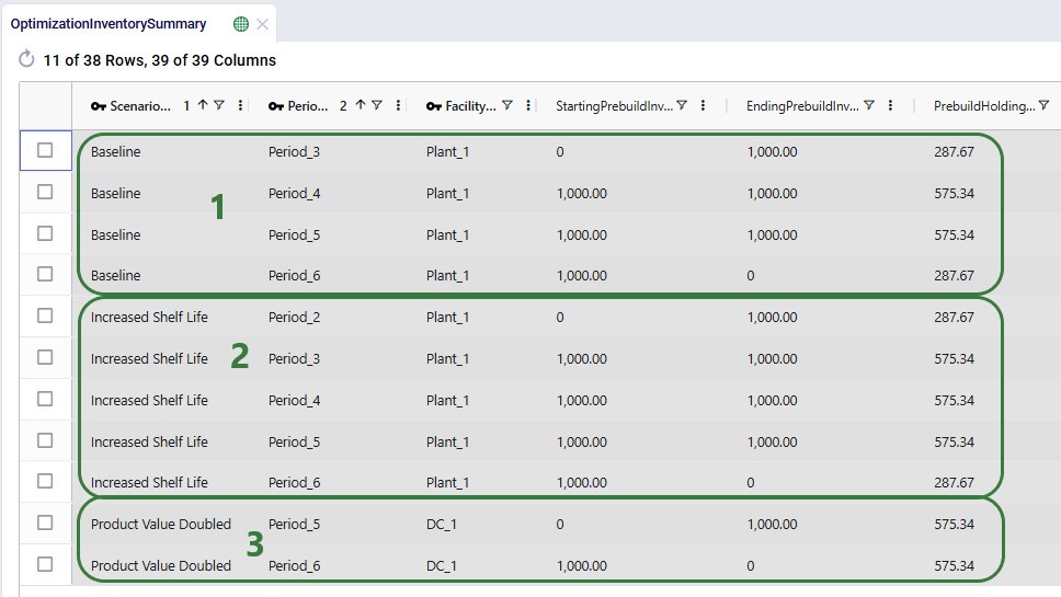
The next screenshot shows the Optimization Inventory Summary filtered for Product_2. Since we know it is produced in different periods for each of the 3 scenarios and that the demand occurs in Period_6, we expect to see the product sitting in inventory for a different number of periods in the different scenarios:
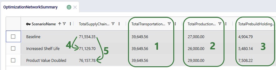
In the Optimization Network Summary output table, we can check the total cost by scenario and how the 3 costs modelled contribute to this total cost:
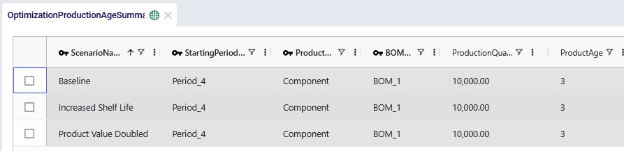
Next, we will take a look at the 3 new output tables, which detail the age of products that are used in production, of products that are transported, and of products that are sitting in inventory. We will start with the Optimization Production Age Summary output table:
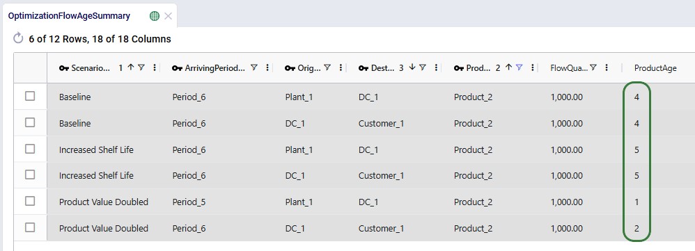
Next, we will look at the age of Product_2 when it is shipped between locations:
Lastly, we will look at 2 screenshots of the new Optimization Inventory Age Summary output table. This first one only looks at the ages of Product_1 and Component at Plant_1 in the Baseline scenario. The values for their inventory levels and ages are the same in the other 2 scenarios as the production of these 2 products occurs during the same periods for all 3 scenarios:

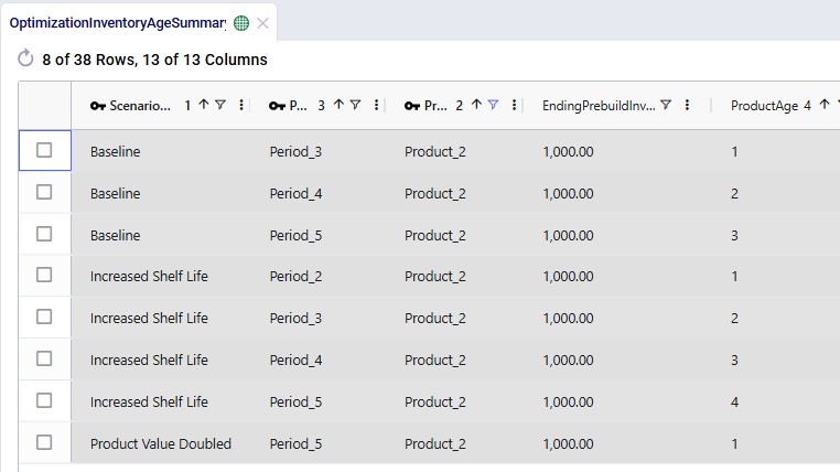
In the next screenshot, we look at the same output table, Optimization Inventory Age Summary, but now filtered for Product_2 and for all 3 scenarios:
For any questions on these new features, please do not hesitate to contact Optilogic support on support@optilogic.com.

Cosmic Frog’s network optimization engine (Neo) can now account for shelf life and maturation time of products out of the box with the addition of several fields to the Products input table. The age of product that is used in production, product which flows between locations, and product sitting in inventory is now also reported in 3 new output tables, so users have 100% visibility into the age of their products across the operations.
In this documentation, we will give a brief overview of the new features first and then walk through a small demo model, which users can copy from the Resource Library, showing both shelf life and maturation time using 3 scenarios.
The new feature set consists of:
Please note that:
We will now showcase the use of both Shelf Life and Maturation Time in a small demo model. This model can be copied to your own Optilogic account from the Resource Library (see also the “How to use the Resource Library” Help Center article). This model has 3 locations which are shown on the map below:
It is a multi-period model with 6 periods, which are each 1 week long (the Model End Date is set to February 12, 2025, on the Model Settings input table, not shown):
There are 3 products included the model: 2 finished goods, Product_1 and Product_2, and 1 raw material, named Component. The component is used in a bill of materials to produce Product_1, as we will see in the screenshots after this one.
As mentioned above, a bill of materials is used to produce finished good Product_1:
This bill of materials is named BOM_1 and it specifies that 10 units of the product named Component are used as an input (product type = Component) of this bill of materials. Note that the bill of materials does not indicate the end product that is produced with it. This is specified by associating production policies with a BOM. To learn more about detailed production modelling using the Neo engine, please see this Help Center article.
In the next screenshot of the production policies table, we see that the plant can produce all 3 products, and that for the production of Product_1, the bill of materials shown in the previous screenshot, BOM_1, is used. The cost per unit is set to 1 here for each product:
For purposes of showing how Shelf Life and Maturation Time work, we will use the Production Policies Multi-Time Period input table too. In here we override the production cost per unit that we just saw in the above screenshot to become increasingly expensive in later periods for all products, adding $1 per unit for each next period. So, to produce a unit of Product_1 in Period_1 costs $1, in Period_2 it costs $2, in Period_3 $3, etc. Same for Component and Product_2:
The production cost is increased here to encourage the model to produce product as early as possible, so that it incurs the lowest possible production cost. It will also still need to respect the shelf life and maturation time requirements. Note that this is also weighed against the increased inventory holding costs for producing earlier than possibly needed, as product will sit in inventory longer if produced earlier. So, the cost differential for production in different periods needs to be sufficiently big as compared to the increased inventory holding cost to see this behavior. We will explore this more through the scenarios that are run in this demo model.
Since products will be spending some time in inventory, we need to have at least 1 inventory policy per product with Stocking Site = True. At the plant, all 3 products can be held in inventory, and there is an initial inventory of 750 units of the Component. At the DC, both finished goods can be held in inventory. The carrying cost percentage to calculate the inventory holding costs is set to 10% for all policies:
Lastly, we will show the demand that has been entered into the Customer Demand table. The customer demands 1,000 units each of the finished goods in period #6:
Other input tables that have populated records which have not been shown in a screenshot above are: Customers, Facilities, and Transportation Policies. The latter specifies that the plant can ship both finished goods to the DC, and the DC can ship both to the customer. The cost of transportation is set to 0.01 per unit per mile on both lanes.
The 3 costs that are modelled are therefore:
There are 3 scenarios run in this model, see also the screenshot below:
The screenshot shows the 3 scenarios on the left, where we see that the Increased Shelf Life and Product Value Doubled scenarios both contain 1 scenario item, whereas the Baseline does not contain any. On the right-hand side, the scenario item of the Increased Shelf Life scenario is shown where we can see that the Shelf Life value of Product_2 is set to 34. See the following Help Center articles for more details on Scenario building and syntax:
Two notes upfront about the outputs before we dive into details as follows:
Now let us first look at when which product is produced through the Optimization Production Summary output table:
The next screenshot shows the Optimization Inventory Summary filtered for Product_2. Since we know it is produced in different periods for each of the 3 scenarios and that the demand occurs in Period_6, we expect to see the product sitting in inventory for a different number of periods in the different scenarios:
In the Optimization Network Summary output table, we can check the total cost by scenario and how the 3 costs modelled contribute to this total cost:
Next, we will take a look at the 3 new output tables, which detail the age of products that are used in production, of products that are transported, and of products that are sitting in inventory. We will start with the Optimization Production Age Summary output table:
Next, we will look at the age of Product_2 when it is shipped between locations:
Lastly, we will look at 2 screenshots of the new Optimization Inventory Age Summary output table. This first one only looks at the ages of Product_1 and Component at Plant_1 in the Baseline scenario. The values for their inventory levels and ages are the same in the other 2 scenarios as the production of these 2 products occurs during the same periods for all 3 scenarios:
In the next screenshot, we look at the same output table, Optimization Inventory Age Summary, but now filtered for Product_2 and for all 3 scenarios:
For any questions on these new features, please do not hesitate to contact Optilogic support on support@optilogic.com.