When a Cosmic Frog model has been built and scenarios of interest have been created, it is usually time to run 1 or multiple scenarios. This documentation covers how scenarios can be kicked off, and which run parameters can be configured by users.
Model Run Screen
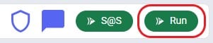
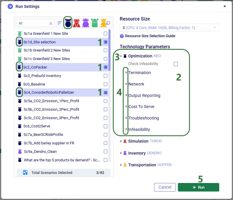
When ready to run scenarios, users can click on the green Run button at the right top of the Cosmic Frog screen:
This will bring up the Run Settings screen:
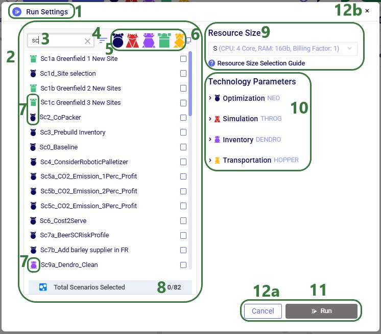
We are on the Run Settings screen.
On the left-hand side of the screen a list of all scenarios contained in the model is shown. Users can select 1 or multiple of these to be run.
To facilitate finding specific scenarios in the list, text can be typed into the search box to filter the scenario list down to scenarios that contain the typed text in their name.
Clicking on this icon with the horizontal bars allows the user to sort the scenario list. Two sort options are available:
Default: the scenarios are listed in the order they were added to the model (i.e. the same order as they are in in the Scenarios module).
A-Z Name: this sorts the scenario list in alphabetical order. Clicking on this sort option again results in sorting the list in reverse alphabetical order.
These are the 5 icons associated with each of the Cosmic Frog engines. From left to right: network optimization (Neo), simulation (Throg), inventory (Dendro), Greenfield (Triad), and transportation optimization (Hopper). These icons are shown here for reference only.
The checkbox at the top of the scenario list can be used to check / un-check all scenarios that are showing in the list simultaneously.
Each scenario has an icon in front of it to show which engine will be used to run this scenario. These match the ones discussed under bullet number 5. The 2 scenario icons outlined in green are a Greenfield and a network optimization scenario, respectively. The other scenario icon outlined in green further down the list is an inventory scenario.
At the bottom of the scenario list the number of selected scenarios is listed. Here none are selected yet.
The user can select the Resource Size that they deem most appropriate for the scenarios to be run with. Larger resource sizes have more CPUs and more RAM available; however, they also have higher billing factors. Therefore, the aim is usually to choose a resource size as small as possible to limit the time billed for running the scenarios, while still being large enough for the scenarios to not run out of memory. More guidance on Resource Size selection and assessment can be found in this help article "Resource Size Selection Guidance"; a link to this article is provided underneath the drop-down list too.
For each engine, run parameters are available for configuration by users. We will go through these for each engine in the following sections of this documentation. Note that no parameters are available here for Greenfield runs; parameters to run Greenfield scenarios are all specified in the Greenfield Settings input table, which are covered in this "Greenfield Settings Explained" Help Center article.
When ready to start running the selected scenario(s), the user can click on the Run button. Note that it is now greyed out and unavailable as no scenarios have been selected. It will be available and green when 1 or more scenarios are selected.
Should the user decide to not run any scenarios at this time, they can close the Run Settings screen without kicking off any runs in 2 ways:
By clicking on the Cancel button. If changes were made to any parameters, these changes will not be saved. In other words, the parameter values will be reverted to those that were there when the Run Settings screen was opened.
By clicking on the x-icon at the right top of the Run Settings screen. If changes were made to any parameters, these changes will be saved.
Please note that:
Scenarios which are run with the same engine will use the same set of parameters when kicked off simultaneously. Should there be a need to run scenarios with different parameters, users currently need to kick them off in separate batches.
Scenarios that are run simultaneously, will currently all use the same selected resource size. Should there be a need to run scenarios using different resource sizes, users currently need to kick them off in separate batches. More to come in future releases!
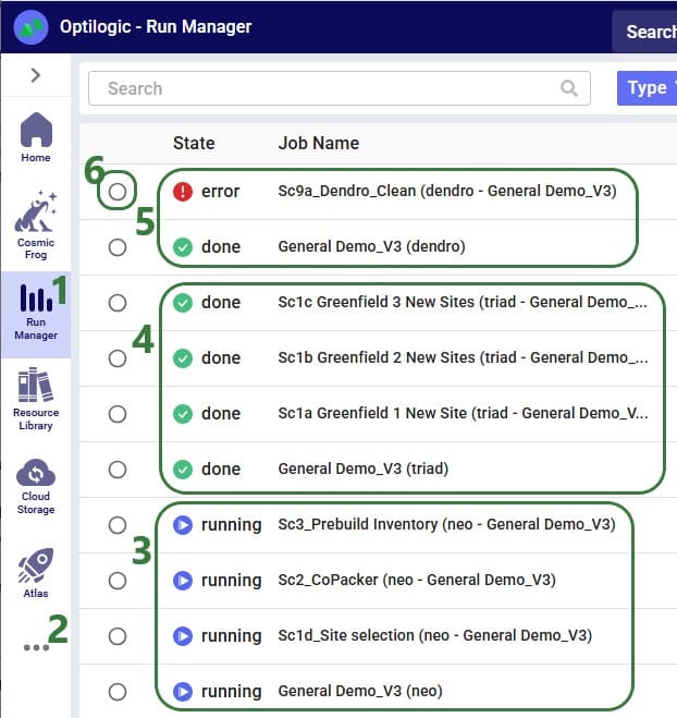
Users can check the progress of all runs in Optilogic's Run Manager application:
To open the Run Manager, click on the Run Manager icon with the vertical bars on the left-hand side of the screen while on the Optilogic platform.
If the Run Manager application is not showing on the left-hand side of the screen, find the icon with the 3 dots and click on it to show all available applications. Then click on Run Manager.
There are 4 jobs listed here which, from bottom to top, are the overall job "General Demo_V3 (neo)" of kicking off network optimization (Neo) scenarios in the model named General Demo_V3. Three scenarios have been kicked off and are currently still running as their State = "running": Sc1d_Site selection, Sc2_CoPacker, and Sc3_Prebuild Inventory.
There are 4 jobs listed here which, from bottom to top, are the overall job "General Demo_V3 (triad)" of kicking off Greenfield (Triad) scenarios in the model named General Demo_V3. Three scenarios have been kicked off and have finished running as their State = "done": Sc1a_Greenfield 1 New Site, Sc1b_Greenfield 2 New Sites, and Sc1c_Greenfield 3 New Sites.
There are 2 jobs listed here which, from bottom to top, are the overall job "General Demo_V3 (dendro)" of kicking off inventory (Dendro) scenarios in the model named General Demo_V3. One scenario has been kicked off and has not completed successfully as its State = "error": Sc9a_Dendro_Clean.
When selecting an individual job by clicking on the circle to the left of it, additional details of the run can be viewed on the right-hand side (not shown in screenshot). This includes job info, job (error) logs, job resource usage metrics, etc.
Not shown in the screenshot above, but if a user wants to end a run, for example in case it was kicked off accidentally or it has been running for a long time without finishing, the user can right-click on the job and choose "Cancel Job" from the context menu.
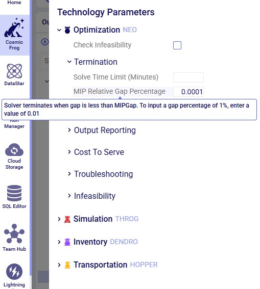
While we will discuss all parameters for each technology in the next sections of the documentation, please note that you can also find short explanations for each of them within Cosmic Frog: when hovering over a parameter, a tooltip explaining the parameter will be shown. In the next screenshot, the user has expanded the Termination section within the Optimization (Neo) technology parameters section and is hovering with the mouse over the "MIP Relative Gap Percentage" parameter, which brings up the tooltip explaining this parameter:
When selecting one or multiple scenarios to be run with the same engine, the corresponding technology parameters are automatically expanded in the Technology Parameters part of the Run Settings screen:
3 scenarios are selected in the scenario list; they are all optimization (Neo) scenarios.
When one or multiple optimization scenarios are selected in the list, the Optimization section in the Technology Parameters part of the Run Settings screen is automatically expanded.
Users can manually expand/collapse these parameter sections by clicking on the caret icons.
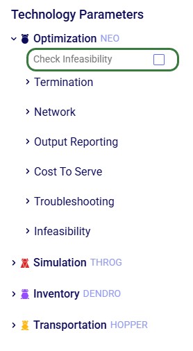
In the Optimization section of the Technology Parameters part of the Run Settings screen, there is 1 general parameter (Check Infeasibility) and 6 additional categories of optimization parameters: Termination, Network, Output Reporting, Cost To Serve, Troubleshooting, and Infeasibility. These sections can also be expanded/collapsed using the caret icons. We will cover each section and their parameters in the next sections of this documentation.
Note that the Run button can now be clicked on and has turned green as 3 scenarios have been selected in the scenario list.
Optimization (Neo) Parameters
When enabled, the Check Infeasibility tool will run an infeasibility diagnostic on the model in order to identify any cause(s) of the scenario being infeasible rather than optimizing the scenario for minimal cost. For more information on using the check infeasibility tool, please see this Help Center article.
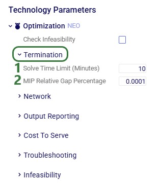
Optimization (Neo) – Termination Parameters
Solve Time Limit (Minutes) – specifies the maximum amount of time the scenario is allowed to run. This is set in minutes.
If a feasible solution where the MIP Relative Gap Percentage (see bullet #2 below) has been reached is found before the Solve Time Limit is reached, the run will stop and this solution is returned. In this case the allowed time is not necessarily used up entirely.
If the MIP Relative Gap Percentage has not been reached within the allowed time, but a feasible solution with a higher gap has been found, this solution will be returned.
If no feasible solution has been found within the allowed time, the scenario run will end without returning results.
The default is blank, meaning scenarios will run until a solution is found that reaches the MIP Relative Gap Percentage, see bullet 2 below.
In case needed, scenarios can always be manually stopped by cancelling the job in the Run Manager application, as explained above.
MIP Relative Gap Percentage – once the difference (gap) between the best bound and currently best-found solution is less than this defined gap, the solver terminates, and the solution is returned as the solution. To set a value of 1%, enter 0.01. The default is set to 0.0001, meaning 0.01%.
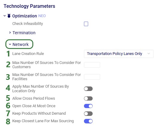
Optimization (Neo) – Network Parameters
Lane Creation Rule – this parameter dictates how the transportation policies and sourcing policies (Customer Fulfillment Policies, Replenishment Policies, Procurement Policies, and Return Policies) input tables are used to create the lanes (origin-destination pairs) that are considered during the optimization. Options are:
Transportation Policy Lanes Only: lanes are only created based on the origin-destination pairs specified in the Transportation Policies input table. This is the default setting for this parameter.
Sourcing Policy Lanes Only: lanes are only created based on the origin-destination pairs specified in the Sourcing Policies input tables (which are: Customer Fulfillment Policies, Replenishment Policies, Procurement Policies, and Return Policies).
Intersection: lanes are created for those origin-destination pairs that exist in both the Transportation Policies and Sourcing Policies input tables.
Union: lanes are created for all origin-destination pairs that exist in the Transportation Policies table and the Sourcing Policies input tables.
Max Number Of Sources To Consider For Customers – when set, this adds constraints to the model where individual customers cannot source from more than this number of sources. It depends on the "Apply Max Number Of Sources By Location Only" parameter setting (see bullet 4 below) if this constraint is applied over the entire model horizon and over all products and modes together (the default behavior when this parameter is off) or for each product-mode-period combination at that location. The sources are evaluated based on distance. For example, if 5 sources are set up for a certain customer in the model, and this parameter is set to 2, then out of those 5 sources, only the 2 that are closest in distance to the customer are considered as sources. The default is blank, meaning that all sources that are set up in the model are kept.
Max Number Of Sources To Consider For Facilities – when set, this adds constraints to the model where individual facilities cannot source from more than this number of sources. It depends on the "Apply Max Number Of Sources By Location Only" parameter setting (see bullet 4 below) if this constraint is applied over the entire model horizon and over all products and modes together (the default behavior when this parameter is off) or for each product-mode-period combination at that location. The sources are evaluated based on distance. For example, if 3 sources are set up for a certain facility in the model, and this parameter is set to 1, then out of those 3 sources, only the 1 that is closest in distance to the facility is considered as a source. The default is blank, meaning that all sources that are set up in the model are kept.
Apply Max Number Of Sources By Location Only – when values are set for the previous 2 parameters, this parameter specifies if those max number of sources parameters are applied for each product-mode-period combination at that location or over all product-mode-period mode combinations together. When this parameter is off (the default), the max number of sources parameters will limit the number of sources for each destination across all product-mode-period combinations. When this parameter is turned on, the max number of sources parameters will limit the number of sources for each unique destination-product-mode-period combination.
Allow Cross Period Flows – turn this parameter on when flows that depart in one period and arrive in a later one need to be allowed in the model. This can be the case when (some) transport times are longer than the length of the periods in the model. By default, this parameter is off, and flows will depart and arrive in the same period regardless of the transport times specified in the model.
Open Close At Most Once – when turned on (the default), facilities and work centers which can be opened and/or closed during the model horizon are not allowed to change status more than once during the model horizon. When turned off, facilities and work centers are allowed to change between open and close states an unlimited number of times during the model horizon.
Keep Products Without Demand – when this option is turned off (the default), products for which no demand exists in the model will be entirely excluded from the model run. When turned on, these products will be included. This can affect the model results, for example:
If there is initial inventory present for the product: inventory holding costs can be incurred and the product will take up storage space and count toward pre-build inventory.
If there are min/fixed production or flow constraints for the product: these will need to be fulfilled, so production, transportation, and inventory holding costs can be incurred in this case, while the product also takes up space and counts towards pre-build inventory.
Keep Closest Lane For Max Sourcing – when this option is turned on (the default), if all sources where a max sourcing range is applied (set in the Max Sourcing Range fields of the Customer Fulfillment Policies, Replenishment Policies, and Procurement Policies tables) fall outside of this sourcing range, the closest source will be kept. When turned off, if all sources where a max sourcing range is applied fall outside of the range, this can lead to the model becoming infeasible if the destination location has no other way of receiving the product(s) it requires to fulfill demand or other model constraints.
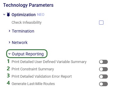
Optimization (Neo) – Output Reporting Parameters
Print Detailed User Defined Variable Summary – when turned on, the Optimization User Defined Variable Summary and Optimization User Defined Variable Term Summary output tables are populated with all outputs related to user defined variables, including records with value of 0. When turned off (the default) these output table are only populated with non-0 values.
Print Constraint Summary – when turned on, the Optimization Constraint Summary output table will be populated, whereas when this parameter is turned off (the default) it will not be populated. As this table can contain a lot of records, it can be helpful to turn it off and only turn it on for troubleshooting purposes or for select scenarios to review how close some constraints are to maxing out for example.
Print Detailed Validation Error Report – when this option is turned off (the default), the Optimization Validation Error Report output table will group the found validation errors by type. When turned on, this table will have individual records for each instance of a validation error. For more information on the Validation Error Report output table, please see "Understanding the Validation Error Report" and "Troubleshooting with Validation Errors".
Generate Last-Mile Routes – when this option is turned on, the Hopper (transportation optimization) engine will be run once the Neo (network optimization) run is complete. This will generate last mile multi-stop routes based on the Neo assignments on this last leg and all Hopper output tables will be populated in addition to the Neo output tables. To learn more about this option to run "Hopper after Neo", please see "Network Transportation Optimization (Neo & Hopper)".
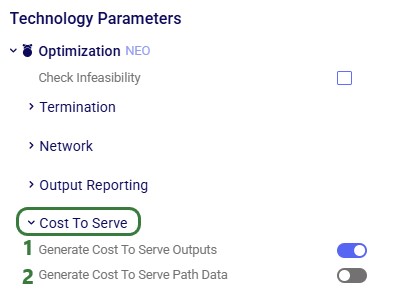
Optimization (Neo) – Cost To Serve Parameters
For more details on the Cost To Serve output tables that are populated by turning the options discussed below on, please see this "Cost to Serve Outputs (Optimization)" Help Center article.
Generate Cost To Serve Outputs – when this option is turned on (the default), the high-level Optimization Cost To Serve Summary output table will be populated after a scenario run. It is not populated when this option is turned off.
Generate Cost To Serve Path Data – when this option is turned on, the Optimization Cost To Serve Path Summary and Optimization Cost To Serve Path Segment Details output tables will be populated. Please note that:
The "Generate Cost To Serve Outputs" option (see bullet 1 above) needs to be turned on when turning this option on.
Turning this option on can add significant time to the output processing as many records may need to be generated for especially the Optimization Cost To Serve Path Segment Details output table, which affects the overall runtime of a scenario.
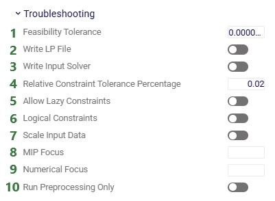
Optimization (Neo) – Troubleshooting Parameters
Feasibility tolerance – since numbers have finite precision on digital computers, sometimes constraints cannot be met exactly. Therefore, the feasibility tolerance sets a limit on the amount of violation allowed on a constraint while still considering it "satisfied". The default value is 0.000001, and for most models users will not need to change this. Should a user suspect a model turns infeasible due to slight constraint violation, they can test this out by relaxing the feasibility tolerance and setting it to a higher value, e.g. try 0.00001 first, then 0.0001, etc.
Write LP (linear program) File – when turned on, this will produce a file containing the linear programming formulation of the model that is being optimized. Experienced users may be able to review this for troubleshooting purposes, and Optilogic's support team may ask for this when troubleshooting any models. The LP-file can be found in the Explorer application: My Files > debug_data > model_name > scenario_name > NEO.lp. By default, this option is turned off. The next screenshot a bit further below shows where the NEO.lp file can be found when running a scenario with this parameter turned on.
Write Input Solver – when turned on, this will write all the data of the input tables that are used during the scenario run into .csv-files. This means that following have been applied before writing these files: scenario changes, excluded records are removed, and records using groups/named table filters are enumerated into records for the individual group/filter members (for groups used in constraints tables only if the group behavior field is set to enumerate). The .csv-files can be found in Explorer > My Files > debug_data > model_name > scenario_name > input_solver, see the screenshot a bit further below. By default, this option is turned off.
Relative Constraint Tolerance Percentage – constraints of type "Fixed With Tolerance" are relaxed by this amount. The default of 0.02 means a relaxation of 2%. For example, if a constraint of type "Fixed With Tolerance" is set to a constraint value of 500, then with a Relative Constraint Tolerance Percentage of 0.02 (2%), values from 490 up to 510 are accepted as satisfying the constraint.
Allow Lazy Constraints – when this option is turned on, constraints that are computationally expensive are at first turned off during the optimization and are added back in later in the process, so they are still respected in the final solution. By default, this option is turned off as it can slow the optimization down. Users are advised to turn it on when a performance issue is detected on a model, in which case it may be able to speed up the optimization.
Logical Constraints – if a model is poorly scaled (for example due to having both very small and very large demand quantities or cost numbers in it), turning this option on may prevent numerical issues leading to infeasibility of the model. Model runtime can however increase when this option is used. By default, this option is turned off.
Scale Input Data – when this option is turned on input data will be scaled; this can help to resolve numeric stability issues in models that contain a large range of numbers.
MIP Focus – the MIP Focus parameter allows you to modify your high-level solution strategy, depending on your goals. By default, the Gurobi MIP solver strikes a balance between finding new feasible solutions and proving that the current solution is optimal. If you are more interested in finding feasible solutions quickly, you can select MIP Focus=1. If you believe the solver is having no trouble finding good quality solutions, and wish to focus more attention on proving optimality, select MIP Focus=2. If the best objective bound is moving very slowly (or not at all), you may want to try MIP Focus=3 to focus on the bound.
Numerical Focus – the Numerical Focus parameter controls the degree to which the engine attempts to detect and manage numerical issues. The default setting (0) makes an automatic choice, with a slight preference for speed. Settings 1-3 increasingly shift the focus towards being more careful in numerical computations. With higher values, the code will spend more time checking the numerical accuracy of intermediate results, and it will employ more expensive techniques in order to avoid potential numerical issues.
Run Preprocessing Only – when this option is turned on, the scenario will first undergo preprocessing (i.e. applying scenario items, expanding groups into individual members, etc.) and then the Integrity Checker is run on the scenario. The results of the integrity checker can then be found in the Optimization Validation Error Report output table. No actual optimization is run when this option is turned on.
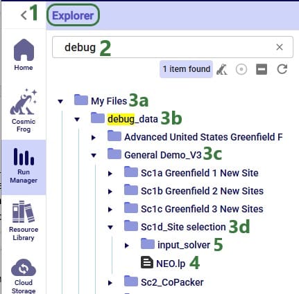
The following screenshot shows where the NEO.lp file can be found when running a scenario with the Write LP File parameter (bullet 2 under the above screenshot) turned on:
While in any application on the Optilogic platform, users can open/close the Explorer by clicking on the caret icon at the top left of the screen.
To quickly find the NEO.lp file, we can search for "debug" in the search box.
The file we are looking for is located in:
The folder "My Files"
The sub-folder "debug_data"
The sub-folder with the name of the model, in this case "General Demo_V3"
The sub-folder with the name of the scenario, in this case "Sc1d_Site selection"
The NEO.lp file in this folder is the file containing the linear programming formulation of this scenario.
The input_solver sub-folder contains the .csv files that are generated when the parameter "Write Input Solver" (see bullet 3 under the previous screenshot) is turned on.
Optimization (Neo) – Infeasibility Parameters
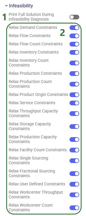
Print Full Solution During Infeasibility Diagnosis - when this option is turned on, the full solution of the model during an infeasibility diagnosis run will be printed. This includes standard output tables (i.e. OptimizationNetworkSummary, OptimizationFlowSummary, OptimizationConstraintSummary, etc.). This option only works when running the Check Infeasibility tool, which needs to be turned on (see further above). When not turned on (the default), only the Optimization Constraint Summary output table is populated when running the Check Feasibility tool on a scenario.
Relax … Constraints – when these options are turned on (by default they all are), the type of constraint described by the option's name will be allowed to be relaxed during a Check Infeasibility run. When turned off, the constraints of that type still need to be satisfied during a Check Infeasibility run. This can help users pinpoint infeasibility in models where many different types of constraints are applied and prioritize which constraints have to be adhered to vs others which may be nice to have satisfied. From the top, these constraints are specified in following input tables:
Demand Constraints – Customer Demand and Facility Demand tables
Single Sourcing Constraints – Customers table (Single Source field, when set to True), Customer Fulfillment Policies table (Optimization Policy field, when set to Single Source), Replenishment Policies table (Optimization Policy field, when set to Single Source), Procurement Policies table (Optimization Policy field, when set to Single Source), Return Policies table (Optimization Policy field, when set to Single Destination)
Fractional Sourcing Constraints –Customer Fulfillment Policies table (Optimization Policy field, when set to By Ratio), Replenishment Policies table (Optimization Policy field, when set to By Ratio), Procurement Policies table (Optimization Policy field, when set to By Ratio), Return Policies table (Optimization Policy field, when set to By Ratio)
User Defined Constraints – User Defined Constraints table
Workcenter Throughput Constraints – Work Centers table (Minimum Throughput and Throughput Capacity fields)
As more types of constraints are added to the Neo engine on an ongoing basis, not all may be captured by one of the above "Relax … Constraints" buckets. Any such constraints, like for example shelf life, are always relaxed when running the Infeasibility Check and, if they are the cause of infeasibility, reported in the Optimization Constraint Summary output table.
Simulation (Throg) Parameters
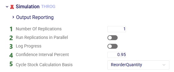
Number Of Replications – for simulation models that use variability in their inputs, multiple replications where different values are used for the variable inputs can be run. This can inform users on how robust a network is: out of all the replications run, how many show a well-functioning network in terms of cost, service and risk and how many do not? Running 20-30 replications is generally a good number to start with, keeping in mind that the more variable the input data is, the more replications should be used.
Run Replications in Parallel – when turned on, multiple replications will be run simultaneously rather than sequentially.
Log Progress – when turned on, a record will be printed in the job log of the simulation run for each day of the simulation horizon. See the next screenshot below on where to find this log. This can help users troubleshoot issues. For example, if a simulation run takes longer than expected, users can review the Job Log to see if it gets stuck on any particular day during the modelling horizon.
Confidence Interval Percent – the confidence interval used for calculating half-width statistics. The default is set to 0.95 (95%).
Cycle Stock Calculation Basis – this parameter controls how cycle stock is calculated for products in the model. If ReorderQuantity is selected (the default), the average cycle stock will be reported as ReorderQuantity / 2. If SafetyStock is selected, the average cycle stock will be reported as AverageInventory - SafetyStock.
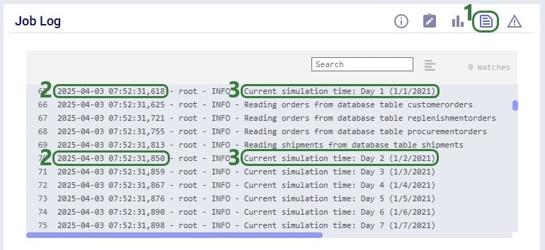
The following screenshot shows part of a Job Log of a simulation run, see also bullet 3 above:
Select the simulation run of interest in the Run Manager application on the Optilogic platform and choose to view the Job Log by clicking on the 4th icon at the top right of the screen.
The current date and time are printed for each record printed in the Job Log.
The current simulation time is printed, a record for each day of the simulation is included.
Simulation (Throg) – Output Reporting Parameters
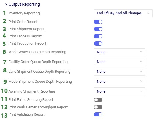
Inventory Reporting – choose whether and, if so, in what way the Simulation Inventory On Hand Report output table will be populated after a simulation run. Options are:
End of Day Only: a record is printed for each facility-product combination at the end of each day.
All Changes Only: a record is printed for facility-product combinations every time the inventory level changes.
End of Day and All Changes: records are printed for each facility-product combination at the end of each day and also every time the inventory level changes. This is the default setting.
None – the Simulation Inventory On Hand Report output table is not populated.
Print Order Report – when turned on (the default), the Simulation Order Report output table will be populated after a simulation run. This table tracks orders at all levels of the supply chain, e.g. production orders, replenishment orders, and customer orders. Users can see when a production order dropped, started, and was completed. For replenishment orders, users can see when they dropped, and when they were filled. If an order is (partially) cancelled, that will be indicated in this table too.
Print Shipment Report – when turned on (the default), the Simulation Shipment Report output table will be populated after a simulation run. All product movements are captured in this table, including what time the shipment departed, when it arrived, and what the due date was (if applicable).
Print Process Report – when turned on (the default), the Simulation Process Report output table will be populated after a simulation run. If any production, (un)loading), or (de)stocking processes are used in the simulation model, the details of when which process was used for what amount of product and time can be found in this output table.
Print Production Report – when turned on (the default), the Simulation Production Report output table will be populated after a simulation run. All productions of the simulation run are detailed in this output table, including start and end time, quantities, and cost associated with the production.
Work Center Queue Depth Reporting – this parameter sets whether and, if so, with what data the Simulation Work Center Queue Depth Report output table will be populated after a simulation run. This queue depth report lists how many items there are in the queue waiting for a specific work center to become available at specific times. Options are:
End of Day Only: a record is printed for each queue at the end of each day.
All Changes Only: a record is printed for queues every time the queue depth changes.
End of Day and All Changes: records are printed for each queue at the end of each day and also every time the queue depth changes.
None – this Simulation Queue Depth Report output table is not populated. This is the default setting.
Facility Order Queue Depth Reporting – this parameter sets whether and, if so, with what data the Simulation Order Fulfillment Queue Depth Report output table will be populated after a simulation run. This queue depth report lists how many items there are in the queue waiting for a specific facility to become available to fulfill an order at specific times. Options are the same as those listed under bullets 6a-d.
Lane Shipment Queue Depth Reporting – this parameter sets whether and, if so, with what data the Simulation Lane Queue Depth Report output table will be populated after a simulation run. This queue depth report lists how many items there are in the queue waiting for a specific lane (origin-destination combination) to become available at specific times. Options are the same as those listed under bullets 6a-d.
Mode Shipment Queue Depth Reporting – this parameter sets whether and, if so, with what data the Simulation Lane Queue Depth Report output table will be populated after a simulation run. This queue depth report lists how many items there are in the queue waiting for a specific mode on a specific lane (origin-destination-mode combination) to become available at specific times. Options are the same as those listed under bullets 6a-d.
Awaiting Shipment Reporting – this parameter sets whether and, if so, with what data the Simulation Awaiting Shipment Report output table will be populated after a simulation run. This report lists the quantity, volume, and weight of specific products at specific facilities which are waiting to be shipped at specific times. Options are the same as those listed under bullets 6a-d.
Print Failed Sourcing Report – this parameter is not currently used by the simulation engine.
Print Work Center Throughput Report – this parameter is not currently used by the simulation engine.
Print Validation Report – when turned on (the default), the Simulation Validation Error Report will be populated after a simulation (Throg) or simulation-optimization (Dendro) run.
Inventory (Dendro) Parameters
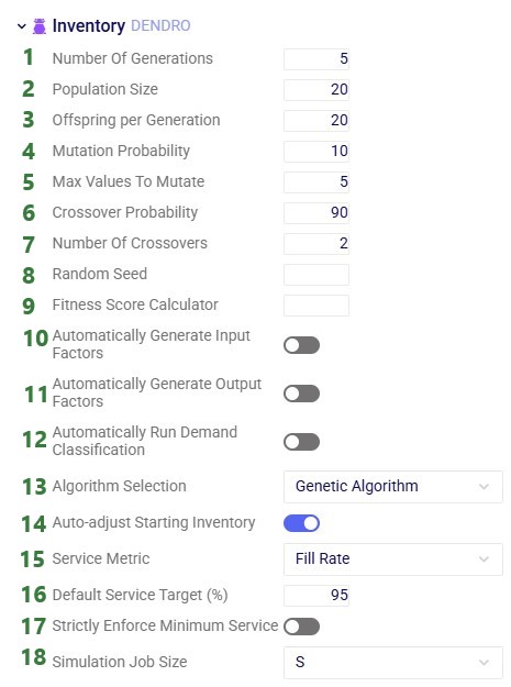
The inventory engine in Cosmic Frog (called Dendro) uses a genetic algorithm to evaluate possible solutions in a successive manner. The parameters that can be set dictate how deep the search space is and how solutions can evolve from one generation to the next. Using the parameter defaults will suffice for most inventory problems, they are however available to change as needed for experienced users.
Number Of Generations – the number of generations the genetic algorithm will go through and calculate. The default value is 5.
Number Of Genes Per Generation – This is the population size, i.e. the number of candidate solutions maintained in the population throughout the algorithm. The default value is 20.
Number Of Offsprings – this specifies how many offsprings are considered from the 2nd until the last generation. This is the number of new candidate solutions created during a step (generation) of the genetic algorithm. The N best solutions from the current population and these offsprings are kept, where N is the population size parameter (Number Of Genes Per Generation, see previous bullet) and then the algorithm moves on to the next step. The default value is 20.
Mutation Probability – the chance that a gene factor will mutate from one generation to the next. The default is 10.
Max Values To Mutate – the maximum number of gene factors that are allowed to mutate from one generation to the next. The default value is 5.
Crossover Probability – the chance that crossover will occur between genes, e.g. genes are swapped. The default value is 90.
Number Of Crossovers – the number of crossover points. The default value is 2.
Random Seed – set the seed of the random number generator of the algorithm to start generating the initial population in an area where optimal solutions are likely to be found. When left blank (the default value), the initial population is generated randomly.
Fitness Score Calculator – available to enable using a customized approach and class name in the code (Optilogic can provide advice and the options for this). When this is left blank (the default value), the data from the Output Factors input table is used.
Automatically Generate Input Factors – automatically populate the Input Factors table before running Dendro. For details on Input Factors, please see the Dendro: Input Factors Guide.
Automatically Generate Output Factors – automatically populate the Output Factors table before running Dendro. For details on Output Factors, please see the Dendro: Output Factors Guide.
Automatically Run Demand Classification – automatically run the Demand Classification utility before running Dendro to calculate reasonable inventory policy values rather than starting from existing ones. Basic Safety Stock logic is used to determine the initial inventory policy for each facility-product combination.
Algorithm Selection – choose which Dendro algorithm to use. Options are:
Genetic Algorithm: Dendro's Genetic Algorithm explores thousands of different inventory policy combinations, simulates each one to see how it performs, and gradually evolves toward the best possible solution. For details on the Genetic Algorithm, please see the Dendro: Genetic Algorithm Guide.
Fast Dendro: A deterministic heuristic that skips the genetic algorithm entirely. Instead of evolving a population, it:
Iteratively adjusts reorder points up/down using a ratio-based heuristic to hit target service levels
Runs one simulation per iteration (not a full population)
Hybrid: Embeds the Fast Dendro heuristic inside the Genetic Algorithm. Specifically:
Runs the Genetic Algorithm (populations, generations, crossover/mutation)
Instead of running a raw simulation for each candidate, it first applies the Fast Dendro heuristic to warm-start/adjust inventory policies before evaluating fitness
Effect: The Genetic Algorithm explores the policy space at a higher level (e.g., which policies to include/exclude, structural choices), while Fast Dendro handles the fine-tuning of reorder point values within each GA evaluation.
Auto-adjust Starting Inventory – when this option is turned on (the default), initial inventory values are automatically adjusted after a Dendro run. Initial inventory will be calculated based on the optimized inventory policies and will be set to S, the order-up-to quantity, for (s,S) policies and to R + Q for (R,Q) policies, where R is the reorder point and Q the reorder quantity.
Service Metric – choose which service level metric to optimize against when using the Fast Dendro algorithm (not applicable to the Genetic Algorithm and Hybrid algorithm options). Options are:
Fill Rate: standard fill rate – percentage of customer demand fulfilled immediately from stock
Ready Rate: measures the probability of having no stockouts
Custom Ready Rate: when this option is selected, Dendro will use facility-product ready rates specified on the Inventory Policies Advanced input table instead of a global value.
OTIF: on-time-in-full rate
Default Service Target (%) – the default target service/level for facility-product combinations that do not have a specific target specified. This option is used for:
When using the Fast Dendro algorithm if target service is not specified in the Inventory Policies Advanced input table.
When automatically generating Input Factors (bullet 10 above) when using the Genetic Algorithm. The default service target value informs how to set ranges on reorder point.
When automatically generating Output Factors (bullet 11 above) when using the Genetic Algorithm. The default service target value informs how to construct the Service output factor.
When automatically running Demand Classification (bullet 12 above) this default service target is used when performing textbook safety stock calculations.
Strictly Enforce Minimum Service – determines policy selection behavior. When turned off (the default), it allows selection of policies which are slightly below the target service level (set by Default Service Target (%), see previous bullet) if they are significantly more cost-efficient. When turned on, the target service level needs to be met or exceeded.
Simulation Job Size – users can choose the resource size for the simulation runs that will be done during each generation of the Dendro algorithm. This can be set independently from the resource size that is selected above the Technology Parameters, which is used for the Parent run job of the model run.
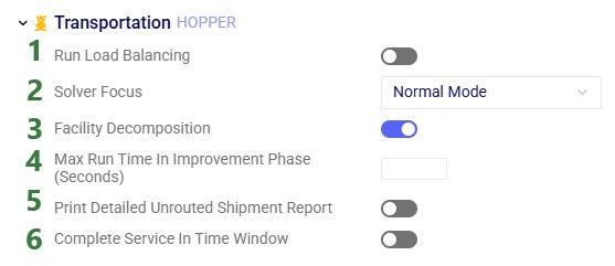
Transportation (Hopper) Parameters
Run Load Balancing – if weekly demand needs to be balanced over a week, the Load Balancing Demand and Load Balancing Schedules input tables can be used to set this up. If both the Shipments table and the Load Balancing Demand/Schedules tables are populated, by default the Shipments table will be used and the Load Balancing Demand/Schedules tables will be ignored. To switch to using the Load Balancing Demand/Schedules tables (and ignoring the Shipments) table, the Run Load Balancing toggle needs to be switched to on (toggle to the left and grey is off; to the right and blue is on).
Solver Focus – controls the solution improvement phase of the solve. Options are:
Normal Mode: uses the standard improvements, usually providing a good balance between finding good solutions and runtime.
Fast Mode: skips the solution improvement phase entirely, providing the fastest runtimes. However, the solutions may be less good as compared to using the other 2 modes.
High Precision Mode: uses a more detailed solution improvement phase. Note that this can lead to longer runtimes.
Facility Decomposition – when this option is turned on (the default), the VRP (Vehicle Routing Problem) is split into multiple subproblems, each associated with a specific facility or depot. The solution process is simplified as compared to trying to solve everything simultaneously, leading to shorter runtimes. If the problem can mathematically be entirely decomposed (e.g. when modelling completely independent facilities used for milk run pick-ups) the results will be very close or the same as when the decomposition option is not used. If this option is used for other problems, like for example interleaved models, it can potentially lead to higher cost solutions.
Max Run Time In Improvement Phase (Seconds) – use this option if you want to put a limit on the time spent by the algorithm in the solution improvement phase. It is set in seconds, so in order to limit this phase to 10 minutes, you need to set this parameter to a value of 600.
Print Detailed Unrouted Shipment Report – when this option is turned on, the Transportation Unrouted Shipment Report output table will be populated. Each record gives an explanation of why a given shipment cannot be inserted into an individual route in the solution. This helps with diagnosis of unrouted shipments, since the reasons might be different for different routes (e.g., capacity exceeded, incompatible time window, breaking of a relationship constraint, etc). The default is off, as the table can get quite large.
Complete Service In Time Window – when this option is turned off (the default), any service time needs to start within the business hours of a stop but is not required to complete within the business hours. Similarly, pickup or delivery of shipments needs to start within the pickup / delivery time windows but does not need to be completed within them. When turned on, any service duration does need to be completed within the location's business hours. This also goes for needing to complete deliveries / pickups within the location's delivery / pickup time windows.
As always, please feel free to contact Optilogic Support at support@optilogic.com in case of questions or feedback.
When a Cosmic Frog model has been built and scenarios of interest have been created, it is usually time to run 1 or multiple scenarios. This documentation covers how scenarios can be kicked off, and which run parameters can be configured by users.
Model Run Screen
When ready to run scenarios, users can click on the green Run button at the right top of the Cosmic Frog screen:
This will bring up the Run Settings screen:
We are on the Run Settings screen.
On the left-hand side of the screen a list of all scenarios contained in the model is shown. Users can select 1 or multiple of these to be run.
To facilitate finding specific scenarios in the list, text can be typed into the search box to filter the scenario list down to scenarios that contain the typed text in their name.
Clicking on this icon with the horizontal bars allows the user to sort the scenario list. Two sort options are available:
Default: the scenarios are listed in the order they were added to the model (i.e. the same order as they are in in the Scenarios module).
A-Z Name: this sorts the scenario list in alphabetical order. Clicking on this sort option again results in sorting the list in reverse alphabetical order.
These are the 5 icons associated with each of the Cosmic Frog engines. From left to right: network optimization (Neo), simulation (Throg), inventory (Dendro), Greenfield (Triad), and transportation optimization (Hopper). These icons are shown here for reference only.
The checkbox at the top of the scenario list can be used to check / un-check all scenarios that are showing in the list simultaneously.
Each scenario has an icon in front of it to show which engine will be used to run this scenario. These match the ones discussed under bullet number 5. The 2 scenario icons outlined in green are a Greenfield and a network optimization scenario, respectively. The other scenario icon outlined in green further down the list is an inventory scenario.
At the bottom of the scenario list the number of selected scenarios is listed. Here none are selected yet.
The user can select the Resource Size that they deem most appropriate for the scenarios to be run with. Larger resource sizes have more CPUs and more RAM available; however, they also have higher billing factors. Therefore, the aim is usually to choose a resource size as small as possible to limit the time billed for running the scenarios, while still being large enough for the scenarios to not run out of memory. More guidance on Resource Size selection and assessment can be found in this help article "Resource Size Selection Guidance"; a link to this article is provided underneath the drop-down list too.
For each engine, run parameters are available for configuration by users. We will go through these for each engine in the following sections of this documentation. Note that no parameters are available here for Greenfield runs; parameters to run Greenfield scenarios are all specified in the Greenfield Settings input table, which are covered in this "Greenfield Settings Explained" Help Center article.
When ready to start running the selected scenario(s), the user can click on the Run button. Note that it is now greyed out and unavailable as no scenarios have been selected. It will be available and green when 1 or more scenarios are selected.
Should the user decide to not run any scenarios at this time, they can close the Run Settings screen without kicking off any runs in 2 ways:
By clicking on the Cancel button. If changes were made to any parameters, these changes will not be saved. In other words, the parameter values will be reverted to those that were there when the Run Settings screen was opened.
By clicking on the x-icon at the right top of the Run Settings screen. If changes were made to any parameters, these changes will be saved.
Please note that:
Scenarios which are run with the same engine will use the same set of parameters when kicked off simultaneously. Should there be a need to run scenarios with different parameters, users currently need to kick them off in separate batches.
Scenarios that are run simultaneously, will currently all use the same selected resource size. Should there be a need to run scenarios using different resource sizes, users currently need to kick them off in separate batches. More to come in future releases!
Users can check the progress of all runs in Optilogic's Run Manager application:
To open the Run Manager, click on the Run Manager icon with the vertical bars on the left-hand side of the screen while on the Optilogic platform.
If the Run Manager application is not showing on the left-hand side of the screen, find the icon with the 3 dots and click on it to show all available applications. Then click on Run Manager.
There are 4 jobs listed here which, from bottom to top, are the overall job "General Demo_V3 (neo)" of kicking off network optimization (Neo) scenarios in the model named General Demo_V3. Three scenarios have been kicked off and are currently still running as their State = "running": Sc1d_Site selection, Sc2_CoPacker, and Sc3_Prebuild Inventory.
There are 4 jobs listed here which, from bottom to top, are the overall job "General Demo_V3 (triad)" of kicking off Greenfield (Triad) scenarios in the model named General Demo_V3. Three scenarios have been kicked off and have finished running as their State = "done": Sc1a_Greenfield 1 New Site, Sc1b_Greenfield 2 New Sites, and Sc1c_Greenfield 3 New Sites.
There are 2 jobs listed here which, from bottom to top, are the overall job "General Demo_V3 (dendro)" of kicking off inventory (Dendro) scenarios in the model named General Demo_V3. One scenario has been kicked off and has not completed successfully as its State = "error": Sc9a_Dendro_Clean.
When selecting an individual job by clicking on the circle to the left of it, additional details of the run can be viewed on the right-hand side (not shown in screenshot). This includes job info, job (error) logs, job resource usage metrics, etc.
Not shown in the screenshot above, but if a user wants to end a run, for example in case it was kicked off accidentally or it has been running for a long time without finishing, the user can right-click on the job and choose "Cancel Job" from the context menu.
While we will discuss all parameters for each technology in the next sections of the documentation, please note that you can also find short explanations for each of them within Cosmic Frog: when hovering over a parameter, a tooltip explaining the parameter will be shown. In the next screenshot, the user has expanded the Termination section within the Optimization (Neo) technology parameters section and is hovering with the mouse over the "MIP Relative Gap Percentage" parameter, which brings up the tooltip explaining this parameter:
When selecting one or multiple scenarios to be run with the same engine, the corresponding technology parameters are automatically expanded in the Technology Parameters part of the Run Settings screen:
3 scenarios are selected in the scenario list; they are all optimization (Neo) scenarios.
When one or multiple optimization scenarios are selected in the list, the Optimization section in the Technology Parameters part of the Run Settings screen is automatically expanded.
Users can manually expand/collapse these parameter sections by clicking on the caret icons.
In the Optimization section of the Technology Parameters part of the Run Settings screen, there is 1 general parameter (Check Infeasibility) and 6 additional categories of optimization parameters: Termination, Network, Output Reporting, Cost To Serve, Troubleshooting, and Infeasibility. These sections can also be expanded/collapsed using the caret icons. We will cover each section and their parameters in the next sections of this documentation.
Note that the Run button can now be clicked on and has turned green as 3 scenarios have been selected in the scenario list.
Optimization (Neo) Parameters
When enabled, the Check Infeasibility tool will run an infeasibility diagnostic on the model in order to identify any cause(s) of the scenario being infeasible rather than optimizing the scenario for minimal cost. For more information on using the check infeasibility tool, please see this Help Center article.
Optimization (Neo) – Termination Parameters
Solve Time Limit (Minutes) – specifies the maximum amount of time the scenario is allowed to run. This is set in minutes.
If a feasible solution where the MIP Relative Gap Percentage (see bullet #2 below) has been reached is found before the Solve Time Limit is reached, the run will stop and this solution is returned. In this case the allowed time is not necessarily used up entirely.
If the MIP Relative Gap Percentage has not been reached within the allowed time, but a feasible solution with a higher gap has been found, this solution will be returned.
If no feasible solution has been found within the allowed time, the scenario run will end without returning results.
The default is blank, meaning scenarios will run until a solution is found that reaches the MIP Relative Gap Percentage, see bullet 2 below.
In case needed, scenarios can always be manually stopped by cancelling the job in the Run Manager application, as explained above.
MIP Relative Gap Percentage – once the difference (gap) between the best bound and currently best-found solution is less than this defined gap, the solver terminates, and the solution is returned as the solution. To set a value of 1%, enter 0.01. The default is set to 0.0001, meaning 0.01%.
Optimization (Neo) – Network Parameters
Lane Creation Rule – this parameter dictates how the transportation policies and sourcing policies (Customer Fulfillment Policies, Replenishment Policies, Procurement Policies, and Return Policies) input tables are used to create the lanes (origin-destination pairs) that are considered during the optimization. Options are:
Transportation Policy Lanes Only: lanes are only created based on the origin-destination pairs specified in the Transportation Policies input table. This is the default setting for this parameter.
Sourcing Policy Lanes Only: lanes are only created based on the origin-destination pairs specified in the Sourcing Policies input tables (which are: Customer Fulfillment Policies, Replenishment Policies, Procurement Policies, and Return Policies).
Intersection: lanes are created for those origin-destination pairs that exist in both the Transportation Policies and Sourcing Policies input tables.
Union: lanes are created for all origin-destination pairs that exist in the Transportation Policies table and the Sourcing Policies input tables.
Max Number Of Sources To Consider For Customers – when set, this adds constraints to the model where individual customers cannot source from more than this number of sources. It depends on the "Apply Max Number Of Sources By Location Only" parameter setting (see bullet 4 below) if this constraint is applied over the entire model horizon and over all products and modes together (the default behavior when this parameter is off) or for each product-mode-period combination at that location. The sources are evaluated based on distance. For example, if 5 sources are set up for a certain customer in the model, and this parameter is set to 2, then out of those 5 sources, only the 2 that are closest in distance to the customer are considered as sources. The default is blank, meaning that all sources that are set up in the model are kept.
Max Number Of Sources To Consider For Facilities – when set, this adds constraints to the model where individual facilities cannot source from more than this number of sources. It depends on the "Apply Max Number Of Sources By Location Only" parameter setting (see bullet 4 below) if this constraint is applied over the entire model horizon and over all products and modes together (the default behavior when this parameter is off) or for each product-mode-period combination at that location. The sources are evaluated based on distance. For example, if 3 sources are set up for a certain facility in the model, and this parameter is set to 1, then out of those 3 sources, only the 1 that is closest in distance to the facility is considered as a source. The default is blank, meaning that all sources that are set up in the model are kept.
Apply Max Number Of Sources By Location Only – when values are set for the previous 2 parameters, this parameter specifies if those max number of sources parameters are applied for each product-mode-period combination at that location or over all product-mode-period mode combinations together. When this parameter is off (the default), the max number of sources parameters will limit the number of sources for each destination across all product-mode-period combinations. When this parameter is turned on, the max number of sources parameters will limit the number of sources for each unique destination-product-mode-period combination.
Allow Cross Period Flows – turn this parameter on when flows that depart in one period and arrive in a later one need to be allowed in the model. This can be the case when (some) transport times are longer than the length of the periods in the model. By default, this parameter is off, and flows will depart and arrive in the same period regardless of the transport times specified in the model.
Open Close At Most Once – when turned on (the default), facilities and work centers which can be opened and/or closed during the model horizon are not allowed to change status more than once during the model horizon. When turned off, facilities and work centers are allowed to change between open and close states an unlimited number of times during the model horizon.
Keep Products Without Demand – when this option is turned off (the default), products for which no demand exists in the model will be entirely excluded from the model run. When turned on, these products will be included. This can affect the model results, for example:
If there is initial inventory present for the product: inventory holding costs can be incurred and the product will take up storage space and count toward pre-build inventory.
If there are min/fixed production or flow constraints for the product: these will need to be fulfilled, so production, transportation, and inventory holding costs can be incurred in this case, while the product also takes up space and counts towards pre-build inventory.
Keep Closest Lane For Max Sourcing – when this option is turned on (the default), if all sources where a max sourcing range is applied (set in the Max Sourcing Range fields of the Customer Fulfillment Policies, Replenishment Policies, and Procurement Policies tables) fall outside of this sourcing range, the closest source will be kept. When turned off, if all sources where a max sourcing range is applied fall outside of the range, this can lead to the model becoming infeasible if the destination location has no other way of receiving the product(s) it requires to fulfill demand or other model constraints.
Optimization (Neo) – Output Reporting Parameters
Print Detailed User Defined Variable Summary – when turned on, the Optimization User Defined Variable Summary and Optimization User Defined Variable Term Summary output tables are populated with all outputs related to user defined variables, including records with value of 0. When turned off (the default) these output table are only populated with non-0 values.
Print Constraint Summary – when turned on, the Optimization Constraint Summary output table will be populated, whereas when this parameter is turned off (the default) it will not be populated. As this table can contain a lot of records, it can be helpful to turn it off and only turn it on for troubleshooting purposes or for select scenarios to review how close some constraints are to maxing out for example.
Print Detailed Validation Error Report – when this option is turned off (the default), the Optimization Validation Error Report output table will group the found validation errors by type. When turned on, this table will have individual records for each instance of a validation error. For more information on the Validation Error Report output table, please see "Understanding the Validation Error Report" and "Troubleshooting with Validation Errors".
Generate Last-Mile Routes – when this option is turned on, the Hopper (transportation optimization) engine will be run once the Neo (network optimization) run is complete. This will generate last mile multi-stop routes based on the Neo assignments on this last leg and all Hopper output tables will be populated in addition to the Neo output tables. To learn more about this option to run "Hopper after Neo", please see "Network Transportation Optimization (Neo & Hopper)".
Optimization (Neo) – Cost To Serve Parameters
For more details on the Cost To Serve output tables that are populated by turning the options discussed below on, please see this "Cost to Serve Outputs (Optimization)" Help Center article.
Generate Cost To Serve Outputs – when this option is turned on (the default), the high-level Optimization Cost To Serve Summary output table will be populated after a scenario run. It is not populated when this option is turned off.
Generate Cost To Serve Path Data – when this option is turned on, the Optimization Cost To Serve Path Summary and Optimization Cost To Serve Path Segment Details output tables will be populated. Please note that:
The "Generate Cost To Serve Outputs" option (see bullet 1 above) needs to be turned on when turning this option on.
Turning this option on can add significant time to the output processing as many records may need to be generated for especially the Optimization Cost To Serve Path Segment Details output table, which affects the overall runtime of a scenario.
Optimization (Neo) – Troubleshooting Parameters
Feasibility tolerance – since numbers have finite precision on digital computers, sometimes constraints cannot be met exactly. Therefore, the feasibility tolerance sets a limit on the amount of violation allowed on a constraint while still considering it "satisfied". The default value is 0.000001, and for most models users will not need to change this. Should a user suspect a model turns infeasible due to slight constraint violation, they can test this out by relaxing the feasibility tolerance and setting it to a higher value, e.g. try 0.00001 first, then 0.0001, etc.
Write LP (linear program) File – when turned on, this will produce a file containing the linear programming formulation of the model that is being optimized. Experienced users may be able to review this for troubleshooting purposes, and Optilogic's support team may ask for this when troubleshooting any models. The LP-file can be found in the Explorer application: My Files > debug_data > model_name > scenario_name > NEO.lp. By default, this option is turned off. The next screenshot a bit further below shows where the NEO.lp file can be found when running a scenario with this parameter turned on.
Write Input Solver – when turned on, this will write all the data of the input tables that are used during the scenario run into .csv-files. This means that following have been applied before writing these files: scenario changes, excluded records are removed, and records using groups/named table filters are enumerated into records for the individual group/filter members (for groups used in constraints tables only if the group behavior field is set to enumerate). The .csv-files can be found in Explorer > My Files > debug_data > model_name > scenario_name > input_solver, see the screenshot a bit further below. By default, this option is turned off.
Relative Constraint Tolerance Percentage – constraints of type "Fixed With Tolerance" are relaxed by this amount. The default of 0.02 means a relaxation of 2%. For example, if a constraint of type "Fixed With Tolerance" is set to a constraint value of 500, then with a Relative Constraint Tolerance Percentage of 0.02 (2%), values from 490 up to 510 are accepted as satisfying the constraint.
Allow Lazy Constraints – when this option is turned on, constraints that are computationally expensive are at first turned off during the optimization and are added back in later in the process, so they are still respected in the final solution. By default, this option is turned off as it can slow the optimization down. Users are advised to turn it on when a performance issue is detected on a model, in which case it may be able to speed up the optimization.
Logical Constraints – if a model is poorly scaled (for example due to having both very small and very large demand quantities or cost numbers in it), turning this option on may prevent numerical issues leading to infeasibility of the model. Model runtime can however increase when this option is used. By default, this option is turned off.
Scale Input Data – when this option is turned on input data will be scaled; this can help to resolve numeric stability issues in models that contain a large range of numbers.
MIP Focus – the MIP Focus parameter allows you to modify your high-level solution strategy, depending on your goals. By default, the Gurobi MIP solver strikes a balance between finding new feasible solutions and proving that the current solution is optimal. If you are more interested in finding feasible solutions quickly, you can select MIP Focus=1. If you believe the solver is having no trouble finding good quality solutions, and wish to focus more attention on proving optimality, select MIP Focus=2. If the best objective bound is moving very slowly (or not at all), you may want to try MIP Focus=3 to focus on the bound.
Numerical Focus – the Numerical Focus parameter controls the degree to which the engine attempts to detect and manage numerical issues. The default setting (0) makes an automatic choice, with a slight preference for speed. Settings 1-3 increasingly shift the focus towards being more careful in numerical computations. With higher values, the code will spend more time checking the numerical accuracy of intermediate results, and it will employ more expensive techniques in order to avoid potential numerical issues.
Run Preprocessing Only – when this option is turned on, the scenario will first undergo preprocessing (i.e. applying scenario items, expanding groups into individual members, etc.) and then the Integrity Checker is run on the scenario. The results of the integrity checker can then be found in the Optimization Validation Error Report output table. No actual optimization is run when this option is turned on.
The following screenshot shows where the NEO.lp file can be found when running a scenario with the Write LP File parameter (bullet 2 under the above screenshot) turned on:
While in any application on the Optilogic platform, users can open/close the Explorer by clicking on the caret icon at the top left of the screen.
To quickly find the NEO.lp file, we can search for "debug" in the search box.
The file we are looking for is located in:
The folder "My Files"
The sub-folder "debug_data"
The sub-folder with the name of the model, in this case "General Demo_V3"
The sub-folder with the name of the scenario, in this case "Sc1d_Site selection"
The NEO.lp file in this folder is the file containing the linear programming formulation of this scenario.
The input_solver sub-folder contains the .csv files that are generated when the parameter "Write Input Solver" (see bullet 3 under the previous screenshot) is turned on.
Optimization (Neo) – Infeasibility Parameters
Print Full Solution During Infeasibility Diagnosis - when this option is turned on, the full solution of the model during an infeasibility diagnosis run will be printed. This includes standard output tables (i.e. OptimizationNetworkSummary, OptimizationFlowSummary, OptimizationConstraintSummary, etc.). This option only works when running the Check Infeasibility tool, which needs to be turned on (see further above). When not turned on (the default), only the Optimization Constraint Summary output table is populated when running the Check Feasibility tool on a scenario.
Relax … Constraints – when these options are turned on (by default they all are), the type of constraint described by the option's name will be allowed to be relaxed during a Check Infeasibility run. When turned off, the constraints of that type still need to be satisfied during a Check Infeasibility run. This can help users pinpoint infeasibility in models where many different types of constraints are applied and prioritize which constraints have to be adhered to vs others which may be nice to have satisfied. From the top, these constraints are specified in following input tables:
Demand Constraints – Customer Demand and Facility Demand tables
Single Sourcing Constraints – Customers table (Single Source field, when set to True), Customer Fulfillment Policies table (Optimization Policy field, when set to Single Source), Replenishment Policies table (Optimization Policy field, when set to Single Source), Procurement Policies table (Optimization Policy field, when set to Single Source), Return Policies table (Optimization Policy field, when set to Single Destination)
Fractional Sourcing Constraints –Customer Fulfillment Policies table (Optimization Policy field, when set to By Ratio), Replenishment Policies table (Optimization Policy field, when set to By Ratio), Procurement Policies table (Optimization Policy field, when set to By Ratio), Return Policies table (Optimization Policy field, when set to By Ratio)
User Defined Constraints – User Defined Constraints table
Workcenter Throughput Constraints – Work Centers table (Minimum Throughput and Throughput Capacity fields)
As more types of constraints are added to the Neo engine on an ongoing basis, not all may be captured by one of the above "Relax … Constraints" buckets. Any such constraints, like for example shelf life, are always relaxed when running the Infeasibility Check and, if they are the cause of infeasibility, reported in the Optimization Constraint Summary output table.
Simulation (Throg) Parameters
Number Of Replications – for simulation models that use variability in their inputs, multiple replications where different values are used for the variable inputs can be run. This can inform users on how robust a network is: out of all the replications run, how many show a well-functioning network in terms of cost, service and risk and how many do not? Running 20-30 replications is generally a good number to start with, keeping in mind that the more variable the input data is, the more replications should be used.
Run Replications in Parallel – when turned on, multiple replications will be run simultaneously rather than sequentially.
Log Progress – when turned on, a record will be printed in the job log of the simulation run for each day of the simulation horizon. See the next screenshot below on where to find this log. This can help users troubleshoot issues. For example, if a simulation run takes longer than expected, users can review the Job Log to see if it gets stuck on any particular day during the modelling horizon.
Confidence Interval Percent – the confidence interval used for calculating half-width statistics. The default is set to 0.95 (95%).
Cycle Stock Calculation Basis – this parameter controls how cycle stock is calculated for products in the model. If ReorderQuantity is selected (the default), the average cycle stock will be reported as ReorderQuantity / 2. If SafetyStock is selected, the average cycle stock will be reported as AverageInventory - SafetyStock.
The following screenshot shows part of a Job Log of a simulation run, see also bullet 3 above:
Select the simulation run of interest in the Run Manager application on the Optilogic platform and choose to view the Job Log by clicking on the 4th icon at the top right of the screen.
The current date and time are printed for each record printed in the Job Log.
The current simulation time is printed, a record for each day of the simulation is included.
Simulation (Throg) – Output Reporting Parameters
Inventory Reporting – choose whether and, if so, in what way the Simulation Inventory On Hand Report output table will be populated after a simulation run. Options are:
End of Day Only: a record is printed for each facility-product combination at the end of each day.
All Changes Only: a record is printed for facility-product combinations every time the inventory level changes.
End of Day and All Changes: records are printed for each facility-product combination at the end of each day and also every time the inventory level changes. This is the default setting.
None – the Simulation Inventory On Hand Report output table is not populated.
Print Order Report – when turned on (the default), the Simulation Order Report output table will be populated after a simulation run. This table tracks orders at all levels of the supply chain, e.g. production orders, replenishment orders, and customer orders. Users can see when a production order dropped, started, and was completed. For replenishment orders, users can see when they dropped, and when they were filled. If an order is (partially) cancelled, that will be indicated in this table too.
Print Shipment Report – when turned on (the default), the Simulation Shipment Report output table will be populated after a simulation run. All product movements are captured in this table, including what time the shipment departed, when it arrived, and what the due date was (if applicable).
Print Process Report – when turned on (the default), the Simulation Process Report output table will be populated after a simulation run. If any production, (un)loading), or (de)stocking processes are used in the simulation model, the details of when which process was used for what amount of product and time can be found in this output table.
Print Production Report – when turned on (the default), the Simulation Production Report output table will be populated after a simulation run. All productions of the simulation run are detailed in this output table, including start and end time, quantities, and cost associated with the production.
Work Center Queue Depth Reporting – this parameter sets whether and, if so, with what data the Simulation Work Center Queue Depth Report output table will be populated after a simulation run. This queue depth report lists how many items there are in the queue waiting for a specific work center to become available at specific times. Options are:
End of Day Only: a record is printed for each queue at the end of each day.
All Changes Only: a record is printed for queues every time the queue depth changes.
End of Day and All Changes: records are printed for each queue at the end of each day and also every time the queue depth changes.
None – this Simulation Queue Depth Report output table is not populated. This is the default setting.
Facility Order Queue Depth Reporting – this parameter sets whether and, if so, with what data the Simulation Order Fulfillment Queue Depth Report output table will be populated after a simulation run. This queue depth report lists how many items there are in the queue waiting for a specific facility to become available to fulfill an order at specific times. Options are the same as those listed under bullets 6a-d.
Lane Shipment Queue Depth Reporting – this parameter sets whether and, if so, with what data the Simulation Lane Queue Depth Report output table will be populated after a simulation run. This queue depth report lists how many items there are in the queue waiting for a specific lane (origin-destination combination) to become available at specific times. Options are the same as those listed under bullets 6a-d.
Mode Shipment Queue Depth Reporting – this parameter sets whether and, if so, with what data the Simulation Lane Queue Depth Report output table will be populated after a simulation run. This queue depth report lists how many items there are in the queue waiting for a specific mode on a specific lane (origin-destination-mode combination) to become available at specific times. Options are the same as those listed under bullets 6a-d.
Awaiting Shipment Reporting – this parameter sets whether and, if so, with what data the Simulation Awaiting Shipment Report output table will be populated after a simulation run. This report lists the quantity, volume, and weight of specific products at specific facilities which are waiting to be shipped at specific times. Options are the same as those listed under bullets 6a-d.
Print Failed Sourcing Report – this parameter is not currently used by the simulation engine.
Print Work Center Throughput Report – this parameter is not currently used by the simulation engine.
Print Validation Report – when turned on (the default), the Simulation Validation Error Report will be populated after a simulation (Throg) or simulation-optimization (Dendro) run.
Inventory (Dendro) Parameters
The inventory engine in Cosmic Frog (called Dendro) uses a genetic algorithm to evaluate possible solutions in a successive manner. The parameters that can be set dictate how deep the search space is and how solutions can evolve from one generation to the next. Using the parameter defaults will suffice for most inventory problems, they are however available to change as needed for experienced users.
Number Of Generations – the number of generations the genetic algorithm will go through and calculate. The default value is 5.
Number Of Genes Per Generation – This is the population size, i.e. the number of candidate solutions maintained in the population throughout the algorithm. The default value is 20.
Number Of Offsprings – this specifies how many offsprings are considered from the 2nd until the last generation. This is the number of new candidate solutions created during a step (generation) of the genetic algorithm. The N best solutions from the current population and these offsprings are kept, where N is the population size parameter (Number Of Genes Per Generation, see previous bullet) and then the algorithm moves on to the next step. The default value is 20.
Mutation Probability – the chance that a gene factor will mutate from one generation to the next. The default is 10.
Max Values To Mutate – the maximum number of gene factors that are allowed to mutate from one generation to the next. The default value is 5.
Crossover Probability – the chance that crossover will occur between genes, e.g. genes are swapped. The default value is 90.
Number Of Crossovers – the number of crossover points. The default value is 2.
Random Seed – set the seed of the random number generator of the algorithm to start generating the initial population in an area where optimal solutions are likely to be found. When left blank (the default value), the initial population is generated randomly.
Fitness Score Calculator – available to enable using a customized approach and class name in the code (Optilogic can provide advice and the options for this). When this is left blank (the default value), the data from the Output Factors input table is used.
Automatically Generate Input Factors – automatically populate the Input Factors table before running Dendro. For details on Input Factors, please see the Dendro: Input Factors Guide.
Automatically Generate Output Factors – automatically populate the Output Factors table before running Dendro. For details on Output Factors, please see the Dendro: Output Factors Guide.
Automatically Run Demand Classification – automatically run the Demand Classification utility before running Dendro to calculate reasonable inventory policy values rather than starting from existing ones. Basic Safety Stock logic is used to determine the initial inventory policy for each facility-product combination.
Algorithm Selection – choose which Dendro algorithm to use. Options are:
Genetic Algorithm: Dendro's Genetic Algorithm explores thousands of different inventory policy combinations, simulates each one to see how it performs, and gradually evolves toward the best possible solution. For details on the Genetic Algorithm, please see the Dendro: Genetic Algorithm Guide.
Fast Dendro: A deterministic heuristic that skips the genetic algorithm entirely. Instead of evolving a population, it:
Iteratively adjusts reorder points up/down using a ratio-based heuristic to hit target service levels
Runs one simulation per iteration (not a full population)
Hybrid: Embeds the Fast Dendro heuristic inside the Genetic Algorithm. Specifically:
Runs the Genetic Algorithm (populations, generations, crossover/mutation)
Instead of running a raw simulation for each candidate, it first applies the Fast Dendro heuristic to warm-start/adjust inventory policies before evaluating fitness
Effect: The Genetic Algorithm explores the policy space at a higher level (e.g., which policies to include/exclude, structural choices), while Fast Dendro handles the fine-tuning of reorder point values within each GA evaluation.
Auto-adjust Starting Inventory – when this option is turned on (the default), initial inventory values are automatically adjusted after a Dendro run. Initial inventory will be calculated based on the optimized inventory policies and will be set to S, the order-up-to quantity, for (s,S) policies and to R + Q for (R,Q) policies, where R is the reorder point and Q the reorder quantity.
Service Metric – choose which service level metric to optimize against when using the Fast Dendro algorithm (not applicable to the Genetic Algorithm and Hybrid algorithm options). Options are:
Fill Rate: standard fill rate – percentage of customer demand fulfilled immediately from stock
Ready Rate: measures the probability of having no stockouts
Custom Ready Rate: when this option is selected, Dendro will use facility-product ready rates specified on the Inventory Policies Advanced input table instead of a global value.
OTIF: on-time-in-full rate
Default Service Target (%) – the default target service/level for facility-product combinations that do not have a specific target specified. This option is used for:
When using the Fast Dendro algorithm if target service is not specified in the Inventory Policies Advanced input table.
When automatically generating Input Factors (bullet 10 above) when using the Genetic Algorithm. The default service target value informs how to set ranges on reorder point.
When automatically generating Output Factors (bullet 11 above) when using the Genetic Algorithm. The default service target value informs how to construct the Service output factor.
When automatically running Demand Classification (bullet 12 above) this default service target is used when performing textbook safety stock calculations.
Strictly Enforce Minimum Service – determines policy selection behavior. When turned off (the default), it allows selection of policies which are slightly below the target service level (set by Default Service Target (%), see previous bullet) if they are significantly more cost-efficient. When turned on, the target service level needs to be met or exceeded.
Simulation Job Size – users can choose the resource size for the simulation runs that will be done during each generation of the Dendro algorithm. This can be set independently from the resource size that is selected above the Technology Parameters, which is used for the Parent run job of the model run.
Transportation (Hopper) Parameters
Run Load Balancing – if weekly demand needs to be balanced over a week, the Load Balancing Demand and Load Balancing Schedules input tables can be used to set this up. If both the Shipments table and the Load Balancing Demand/Schedules tables are populated, by default the Shipments table will be used and the Load Balancing Demand/Schedules tables will be ignored. To switch to using the Load Balancing Demand/Schedules tables (and ignoring the Shipments) table, the Run Load Balancing toggle needs to be switched to on (toggle to the left and grey is off; to the right and blue is on).
Solver Focus – controls the solution improvement phase of the solve. Options are:
Normal Mode: uses the standard improvements, usually providing a good balance between finding good solutions and runtime.
Fast Mode: skips the solution improvement phase entirely, providing the fastest runtimes. However, the solutions may be less good as compared to using the other 2 modes.
High Precision Mode: uses a more detailed solution improvement phase. Note that this can lead to longer runtimes.
Facility Decomposition – when this option is turned on (the default), the VRP (Vehicle Routing Problem) is split into multiple subproblems, each associated with a specific facility or depot. The solution process is simplified as compared to trying to solve everything simultaneously, leading to shorter runtimes. If the problem can mathematically be entirely decomposed (e.g. when modelling completely independent facilities used for milk run pick-ups) the results will be very close or the same as when the decomposition option is not used. If this option is used for other problems, like for example interleaved models, it can potentially lead to higher cost solutions.
Max Run Time In Improvement Phase (Seconds) – use this option if you want to put a limit on the time spent by the algorithm in the solution improvement phase. It is set in seconds, so in order to limit this phase to 10 minutes, you need to set this parameter to a value of 600.
Print Detailed Unrouted Shipment Report – when this option is turned on, the Transportation Unrouted Shipment Report output table will be populated. Each record gives an explanation of why a given shipment cannot be inserted into an individual route in the solution. This helps with diagnosis of unrouted shipments, since the reasons might be different for different routes (e.g., capacity exceeded, incompatible time window, breaking of a relationship constraint, etc). The default is off, as the table can get quite large.
Complete Service In Time Window – when this option is turned off (the default), any service time needs to start within the business hours of a stop but is not required to complete within the business hours. Similarly, pickup or delivery of shipments needs to start within the pickup / delivery time windows but does not need to be completed within them. When turned on, any service duration does need to be completed within the location's business hours. This also goes for needing to complete deliveries / pickups within the location's delivery / pickup time windows.
As always, please feel free to contact Optilogic Support at support@optilogic.com in case of questions or feedback.