DataStar Quick Start: Cost to Serve Analysis & Visualization with Power BI

In this quick start guide we will show how users can seamlessly go from using the Resource Library, Cosmic Frog and DataStar applications on the Optilogic platform to creating visualizations in Power BI. The example covers cost to serve analysis using a global sourcing model. We will run 2 scenarios in this Cosmic Frog model with the goal to visualize the total cost difference between the scenarios by customer on a map. We do this by coloring the customers based on the cost difference.

The steps we will walk through are:

1. Copy a model from the Optilogic Resource Library to the user’s Optilogic account
2. Run 2 Neo (network optimization) scenarios of the copied model in Cosmic Frog
3. Import input and output of the Cosmic Frog model into DataStar
4. Use Leapfrog in DataStar to perform cost to serve analysis through basic pivots and calculations
5. Connect Power BI to the Sandbox of the DataStar project
6. In Power BI, build a map visualization of how customer costs change between the 2 scenarios

Please note that DataStar is currently in the Early Adopter phase, where only users who participate in the Early Adopter program have access to it. DataStar is rapidly evolving while we work towards the General Availability release later this year. For any questions about DataStar or the Early Adopter program, please feel free to reach out to Optilogic’s support team on support@optilogic.com.

Step 1: Copy Model from Resource Library

We will first copy the model named “Global Sourcing – Cost to Serve” from the Resource Library to our Optilogic account (learn more about the Resource Library in this help center article):

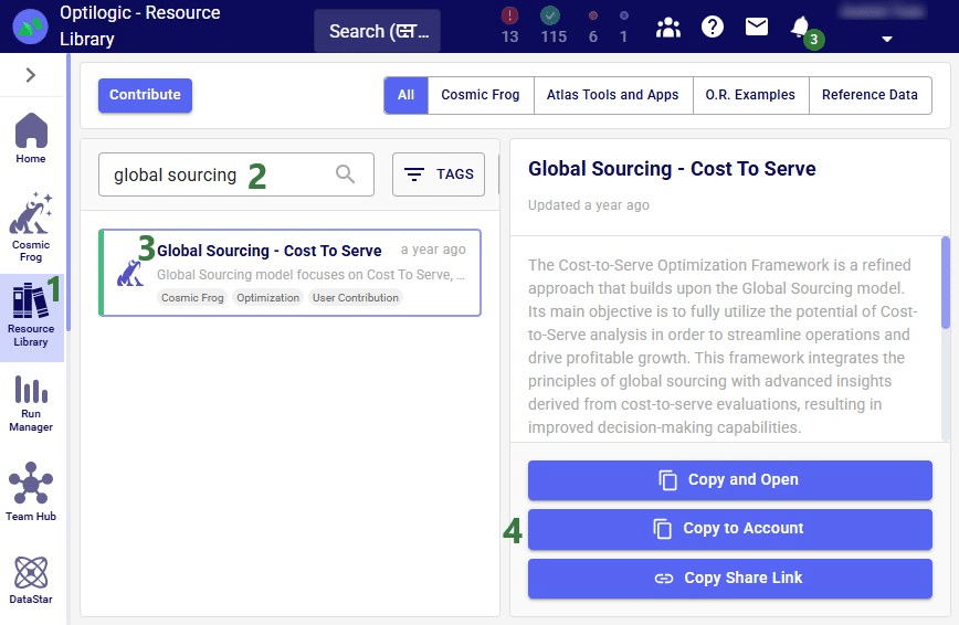
1. On the Optilogic platform, go to the Resource Library application by clicking on its icon in the list of applications on the left-hand side; note that you may need to scroll down. Should you not see the Resource Library icon here, then click on the icon with 3 horizontal dots which will then show all applications that were previously hidden too.
2. In the search box at the top of the Resource Library, type “global sourcing”.
3. The search results in one hit: a Cosmic Frog model named “Global Sourcing – Cost to Serve”. A description of the model will be shown on the right hand-side after clicking on the model to select it.
4. Click on the Copy to Account button on the right-hand side to add a copy of this model to your account.

Step 2: Run Scenarios in Cosmic Frog

Now that the model is in the user’s account, it can be opened in the Cosmic Frog application:

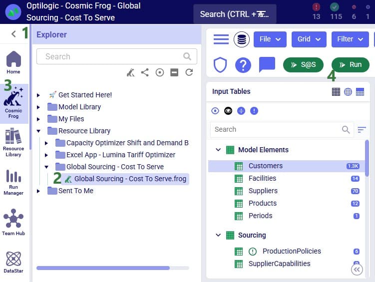
1. Click on the chevron icon at the top left when on the Optilogic platform to expand the Explorer application.
2. You can either search for the model by typing in the Search box at the top of the Explorer or expand the Resource Library folder to find the Global Sourcing – Cost to Server subfolder. This folder contains the model we copied from the Resource Library. Clicking on it will open the model in the Cosmic Frog application.
3. The Cosmic Frog icon is now highlighted as this is the currently active application. We see the Cosmic Frog user interface to the right of the Explorer.
4. Feel free to have a look around in the model, and once ready to run scenarios, click on the green Run button in the toolbar at the top of Cosmic Frog. The Run Settings form comes up:

1. We can select the scenarios to run; we will focus on 2 scenarios: the Baseline and the OpenPotentialFacilities scenarios. Enable their checkboxes so a network optimization (using the Neo engine) will be run on them.
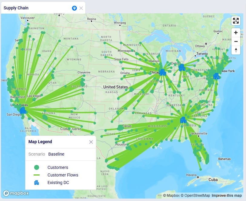
   1. Baseline – this scenario models the as-is network where there are 5 DCs in the US serving around 1.3k customers. Suppliers are located in Europe and China, and a factory in Princeton, Indiana, in the US manufactures all products.
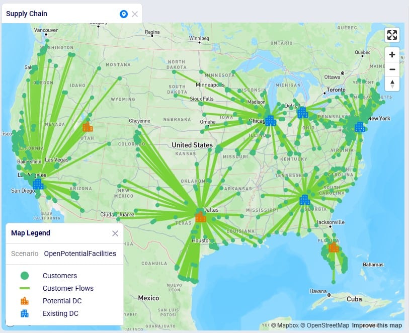
   2. OpenPotentiaFacilities – this scenario considers opening 3 potential DCs, which will weigh the additional startup and fixed operating costs against the decreased transportation costs due to being able to serve customers from DCs closer by.
2. On the right-hand side, expand the Cost to Serve section of the Optimization Technology Parameters, and slide the toggle of the “Generate Cost to Serve Path Data” to the right to turn this setting on. Learn more about cost to serve outputs of Cosmic Frog models in this help center article.
3. Click on the green Run button to kick off the 2 scenarios.

We will only have a brief look at some high-level outputs in Cosmic Frog in this quick start guide, but feel free to explore additional outputs. You can learn more about Cosmic Frog through these help center articles. Let us have a quick look at the Optimization Network Summary output table and the map:

• Optimization Network Summary output table: the total supply chain cost of the OpenPotentialFacilities is reduced by about $4.1M when compared to the Baseline scenario. This is mostly due to a reduction in transportation costs by almost $18M and increase in fixed operating and startup costs of around $14.4M.
• The following 2 screenshots show the DCs, customers, and flows from DCs to customers. This first screenshot is for the Baseline scenario and the second for the OpenPotentialFacilities scenario. We see that of the 3 potential DCs that were considered to be opened in the OpenPotentialFacilities scenario, 2 are being used, 1 in Texas and 1 in Florida.

Step 3: Import Cosmic Frog Tables into DataStar

Our next step is to import the needed input table and output table of the Global Sourcing – Cost to Serve model into DataStar. Open the DataStar application on the Optilogic platform by clicking on its icon in the applications list on the left-hand side. In DataStar, we first create a new project named “Cost to Serve Analysis” and set up a data connection to the Global Sourcing – Cost to Serve model, which we will call “Global Sourcing C2S CF Model”. See the Creating Projects & Data Connections section in the Getting Started with DataStar help center article on how to create projects and data connections. Then, we want to create a macro which will calculate the increase/decrease in total cost by customer between the 2 scenarios. We build this macro as follows:

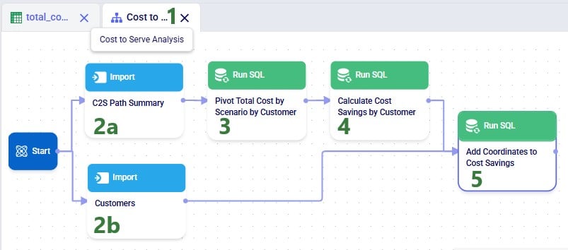
1. The name of the macro created is Cost to Serve Analysis.
2. The first 2 tasks (noted as 2a and 2b in the screenshot) of the macro import tables from the Cosmic Frog model into the Project Sandbox of the DataStar project:
   1. C2S Path Summary – this task imports the Optimization Cost to Serve Path Summary output table from the Global Sourcing – Cost to Serve model into the Project Sandbox. The configuration of this task is shown in the next screenshot. This table will be used to calculate difference in total costs between the 2 scenarios by customer.
   2. Customers – this task imports the Customers input table from the Global Sourcing – Cost to Serve model into the Project Sandbox. To plot the customers on a map, we will need their latitudes and longitudes from this table.
3. We will use Leapfrog to create a Run SQL task named “Pivot Total Cost by Scenario by Customer” that uses the cost to serve path summary table to calculate the total cost by customer for each of the 2 scenarios. This is described in more detail in the ”Step 4” section below.
4. Leapfrog is then used again to create another Run SQL task, “Calculate Cost Savings by Customer” which takes the table created using the task from the previous bullet point and calculates the difference in total costs between the 2 scenarios for each customer. More details on this task can also be found in the “Step 4” section below.
5. In the final Run SQL task of the macro the customers table and the one with the cost increase/decrease by customer (created by the task from the previous bullet point) are joined and the coordinates are added to the cost increase/decrease table. Again, for details see the “Step 4” section below.

The configuration of the first import task, C2S Path Summary, is shown in this screenshot:

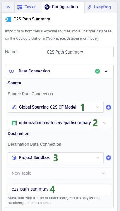
1. As the Source Data Connection, we select the connection to the Global Sourcing – Cost to Serve model, which we have called Global Sourcing C2S CF Model, from the drop-down list.
2. From the tables drop-down list, we select the one named optimizationcosttoservepathsummary.
3. The Destination Data Connection is the Project Sandbox.
4. A new table will be created in the Project Sandbox, and we are naming it c2s_path_summary.

The configuration of the other import task, Customers, uses the same Source Data Connection, but instead of the optimizationcosttoservepathsummary table, we choose the customers table as the table to import. Again, the Project Sandbox is the Destination Data Connection, and the new table is simply called customers.

Step 4: Use Leapfrog in DataStar for Cost to Serve Analysis

Instead of writing SQL queries ourselves to pivot the data in the cost to serve path summary table to create a new table where for each customer there is a row which has the customer name and the total cost for each scenario, we can use Leapfrog to do it for us. See the Leapfrog section in the Getting Started with DataStar help center article and this quick start guide on using natural language to create DataStar tasks to learn more about using Leapfrog in DataStar effectively. For the Pivot Total Cost by Scenario by Customer task, the 2 Leapfrog prompts that were used to create the task are shown in the following screenshot:

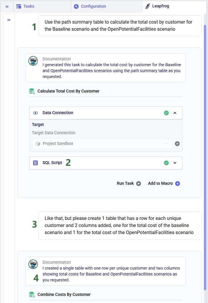
1. The first prompt given to Leapfrog was: “Use the path summary table to calculate the total cost by customer for the Baseline scenario and the OpenPotentialFacilities scenario”.
2. Leapfrog’s response contains a SQL Script (the SQL is not shown in the screenshot). On reviewing this, we find that Leapfrog will create 2 tables, 1 with the total cost by customer for the Baseline scenario and 1 with the total cost by customer for the OpenPotentialFacilities scenario. This is not what we want as we would like to have these costs in 1 table so we can calculate the difference.
3. We follow the first prompt up with this one to steer it to create 1 table instead of 2: “Like that, but please create 1 table that has a row for each unique customer and 2 columns added, one for the total cost of the baseline scenario and 1 for the total cost of the OpenPotentialFacilities scenario”.
4. Leapfrog’s documentation response to this second prompt states that now it has created a single table with the requested 2 columns. The SQL Script is not shown in the screenshot, but it follows here, and upon review we are satisfied that this will achieve what we intend so this task is added to the macro, and is renamed to “Pivot Total Cost by Scenario by Customer”.

The SQL Script reads:

DROP TABLE IF EXISTS total_cost_by_customer_combined;
CREATE TABLE total_cost_by_customer_combined AS
SELECT
  pathdestination AS customer,
  SUM(CASE WHEN scenarioname = 'Baseline' THEN pathcost ELSE 0 END)
    AS total_cost_baseline,
  SUM(CASE WHEN scenarioname = 'OpenPotentialFacilities' THEN pathcost ELSE 0 END)
    AS total_cost_openpotentialfacilities
FROM c2s_path_summary
WHERE scenarioname IN ('Baseline', 'OpenPotentialFacilities')
GROUP BY pathdestination
ORDER BY pathdestination;

To create the Calculate Cost Savings by Customer task, we gave Leapfrog the following prompt: “Use the total cost by customer table and add a column to calculate cost savings as the baseline cost minus the openpotentalfacilities cost”. The resulting SQL Script reads as follows:

ALTER TABLE total_cost_by_customer_combined ADD COLUMN cost_savings DOUBLE PRECISION;
UPDATE total_cost_by_customer_combined SET
  cost_savings = total_cost_baseline - total_cost_openpotentialfacilities;

This task is also added to the macro; its name is “Calculate Cost Savings by Customer”.

Lastly, we give Leapfrog the following prompt to join the table with cost savings (total_cost_by_customer_combined) and the customers table to add the coordinates from the customers table to the cost savings table: “Join the customers and total_cost_by_customer_combined tables on customer and add the latitude and longitude columns from the customers table to the total_cost_by_customer_combined table. Use an inner join and do not create a new table, add the columns to the existing total_cost_by_customer_combined table”. This is the resulting SQL Script, which was added to the macro as the “Add Coordinates to Cost Savings” task:

ALTER TABLE total_cost_by_customer_combined ADD COLUMN latitude VARCHAR;
ALTER TABLE total_cost_by_customer_combined ADD COLUMN longitude VARCHAR;
UPDATE total_cost_by_customer_combined SET latitude = c.latitude
FROM customers AS c
WHERE total_cost_by_customer_combined.customer = c.customername;
UPDATE total_cost_by_customer_combined SET longitude = c.longitude
FROM customers AS c
WHERE total_cost_by_customer_combined.customer = c.customername;

We can now run the macro, and once it is completed, we take a look at the tables present in the Project Sandbox:

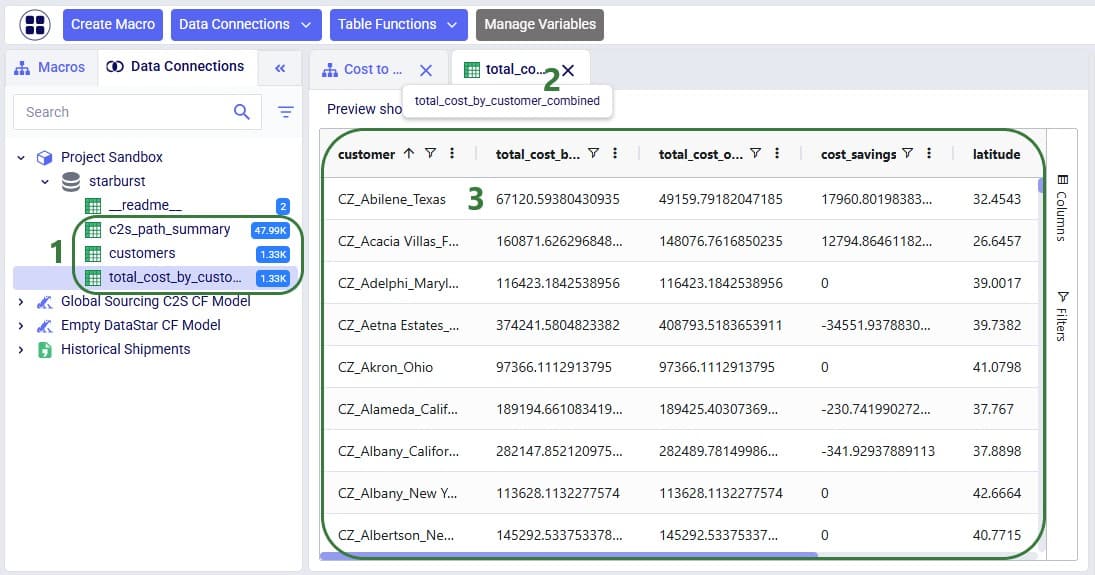
1. Go to the Data Connestions tab, expand the Project Sandbox connection, and then expand the starburst schema. As a result of the macro 3 tables were imported/created in the Project Sandbox: c2s_path_summary, customers, and total_cost_by_customer_combined.
2. Clicking on the total_cost_by_customer_combined table will open it in the central part of DataStar.
3. As was our intention, this table has 1 row for each customer present in the model and columns for the total cost of the customer in the baseline scenario, in the OpenPotentialFacilities table, and the difference between the 2 in the cost_savings column. The latitude and longitude columns have been added too through the join with the customers table (longitude not visible in the screenshot, need to scroll right to see it). We notice that for the first 2 customers (1 in Texas and 1 in Florida) the cost savings are substantial, whereas for the 4^th customer (in Colorado) the total cost in the OpenPotentialFacilities is increased substantially as compared to the Baseline scenario.

Step 5: Connect Power BI to the DataStar Project

We will use Microsoft Power BI to visualize the change in total cost between the 2 scenarios by customer on a map. To do so, we first need to set up a connection to the DataStar project sandbox from within Power BI. Please follow the steps in the “Connecting to Optilogic with Microsoft Power BI” help center article to create this connection. Here we will just show the step to get the connection information for the DataStar Project Sandbox, which underneath is a PostgreSQL database (next screenshot) and selecting the table(s) to use in Power BI on the Navigator screen (screenshot after this one):

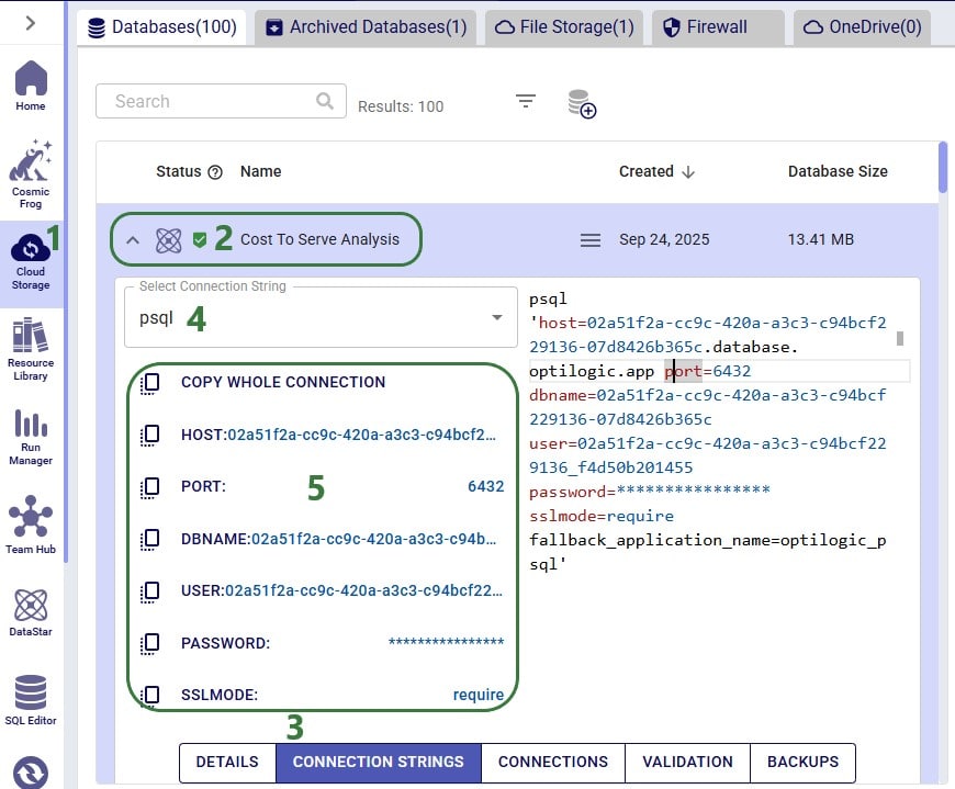
1. On the Optilogic platform, open the Cloud Storage application by clicking on its icon in the list of applications on the left-hand side. Note that it may be in a different position in your list and you may need to scroll. In case it is not listed at all, click on the icon with 3 horizontal dots to show all applications that are currently hidden.
2. On the first tab, Databases, find the database of the DataStar project’s Project Sandbox, which has the same name as the DataStar project. In our case, the name is Cost to Serve Analysis. Note that the icon for DataStar databases is the same as the DataStar application icon, whereas the icon for Cosmic Frog model databases is a frog like the Cosmic Frog application icon. Show the details of the database by clicking on the caret down icon to the left of the DataStar icon, which then changes to a caret up icon.
3. At the bottom, click on the Connection Strings button.
4. In the Select Connection String drop-down list, choose the psql format.
5. The connection information is listed here and can be copied from here when setting up the ODBC connection to the DataStar database in the ODBC Data Sources App.

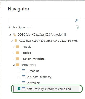
After selecting the connection within Power BI and providing the credentials again, on the Navigator screen, choose to use just the total_cost_by_customer_combined table as this one has all the information needed for the visualization:

Step 6: Power BI Map Visualization

We will set up the visualization on a map using the total_cost_by_customer_combined table that we have just selected for use in Power BI using the following steps:

1. In Power BI, expand the Visualizations and Data panes on the right hand-side.
2. In the Build Visual part of the Visualizations pane, choose Map by clicking on the map icon in the grid of icons.
   1. Note that you may need to enable “Use Map and Filled Map visuals” under File > Options and settings > Options > Security to be able to set up Map visualizations.
3. In the Data pane, expand the total_cost_by_customer_combined table so the columns are visible. Drag the latitude column from here into the Latitude field on the Visualizations pane. Repeat for the longitude column.
4. You can drag the cost_savings and customer columns to the tooltips area, so that these will be shown on hovering over a customer on the map in addition to the latitude and longitude. These can all be renamed as well, if desired, by clicking on the down arrow and choosing the “Rename for this visual” option.
5. At the top of the Visualizations pane, switch to the Format Visual section by clicking on the middle icon.
6. Expand the Bubbles section and then expand the Size section within. Set the size to -6 or another suitable value.
7. In the Bubbles section, expand the Colors section. Click on conditional formatting to open the Default Color – Bubbles – Colors form. In here:
   1. Set Format Style to Gradient.
   2. Set “What field should we base this on?” to cost_savings. Leave Summarization as Sum, and “How should we format empty values?” As zero.
   3. Leave the Minimum and Maximum fields at Lowest Values and Highest Values, respectively. Choose their colors and optionally add a middle color. In our visual below, we have chosen red for the lowest value, and green for the highest value. A middle color was added and its drop-down was changed to Custom, after which 0 was entered as the value. The color for the middle color was set to white.

With the above configuration, the map will look as follows:

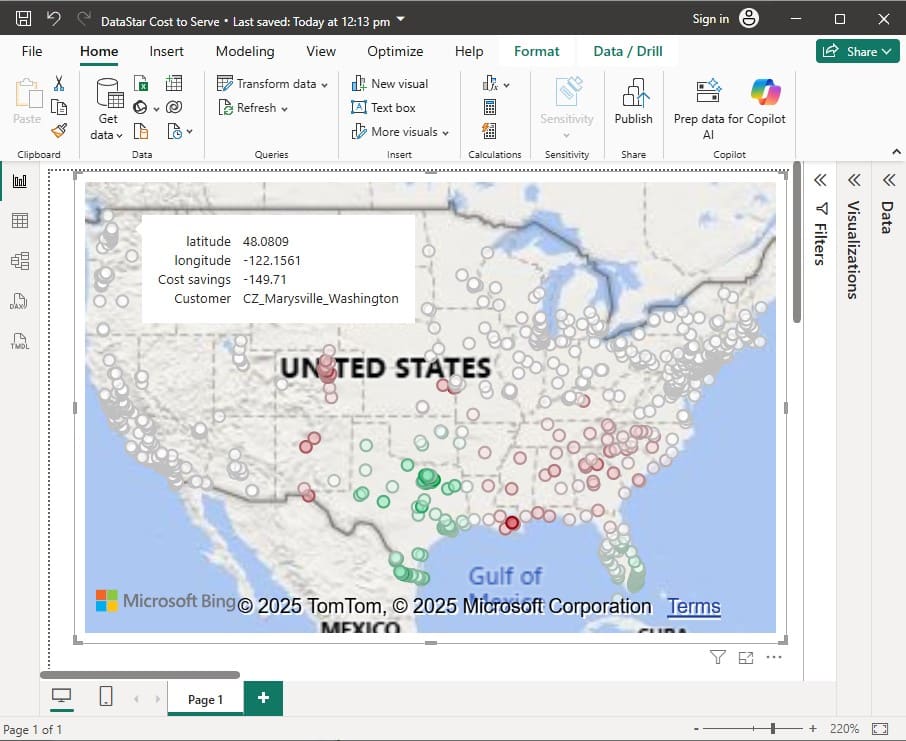
Green customers are those where the total cost went down in the OpenPotentialFacilities scenario, i.e. there are savings for this customer. The darker the green, the higher the savings. White customers did not see a lot of difference in their total costs between the 2 scenarios. The one that is hovered over, in Marysville in Washington state, has a small increase of $149.71 in total costs in the OpenPotentialFacilities scenario as compared to the Baseline scenario. Red customers are those where the total cost went up in the OpenPotentialFacilities scenario (i.e. the cost savings are a negative number); the darker the red, the higher the increase in total costs. As expected, the customers with the highest cost savings (darkest green) are those located in Texas and Florida, as they are now being served from DCs closer to them.

Final Notes

• In this example, we imported the Customers input table of the Cosmic Frog model into the Project Sandbox of the DataStar project. This way, we could use it to get the customers’ latitudes and longitudes added to the table with calculated cost savings by customer. We could have also chosen not to import the Customers table in the DataStar macro and instead set up another ODBC connection to the Cosmic Frog model so we can select the Customers table to use directly in Power BI. The joining of the tables to add the latitudes and longitudes can also be done in Power BI, using the Merge Queries functionality in the Power Query Editor. When using this type of setup, users can then also load in other input / output tables from the Cosmic Frog model itself which can be used for any additional visualizations.
• Here we have used Microsoft Power BI as the third-party tool to use for the map visualization. Other tools, such as Tableau and Alteryx, can be used for visualizations too. To learn more, see the following help center articles:
  • Connecting to Optilogic with Alteryx
  • Connecting to Optilogic with External Data Tools (video)

Helpful Resources

• All available DataStar help center articles can be found in the Navigating DataStar section of the Help Center
• The DataStar Early Access Communityon the Frogger Pond Community portal; accessible for those who participate in the Early Adopter program
• Learn more about using Microsoft Power BI from the Power BI Documentation
• Learn more about using Alteryx from the Help webpage
• Learn more about using Tableau from the Get Started webpage