If you are comfortable with traditional linear programming techniques, you can select the “Write Input Solver Files” and “Write LP File” parameters to get useful output files.

After running, these files are in your file explorer.
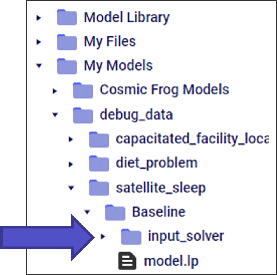
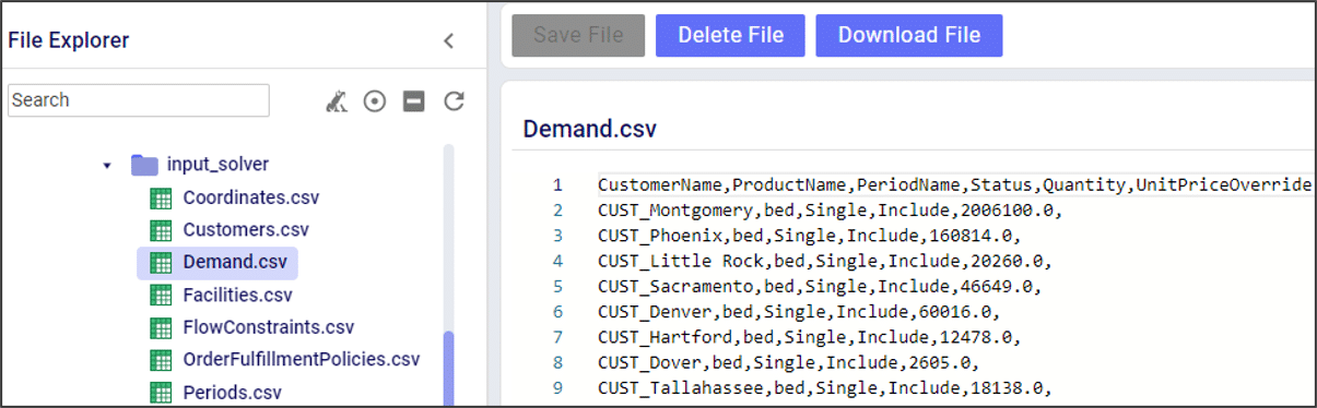
The “input_solver” folder has a list of all the tables that are entered into the optimization solver. This is useful for:
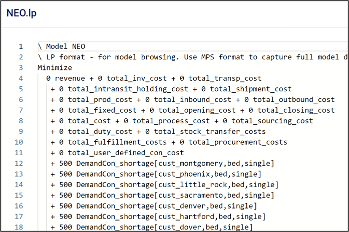
The “model.lp” file shows the model in a more traditional MIP optimization format, including the objective function and model constraints.

When using the Infeasibility Diagnostic engine, the LP file is different than a traditional Neo run. In this case, the cost coefficients in the objective function are set to 0. Instead, a positive cost coefficient is added to each slack constraint, and the goal of the model is to minimize the slack values. This allows us to find the “edge” of infeasibility.

If you are comfortable with traditional linear programming techniques, you can select the “Write Input Solver Files” and “Write LP File” parameters to get useful output files.
After running, these files are in your file explorer.
The “input_solver” folder has a list of all the tables that are entered into the optimization solver. This is useful for:
The “model.lp” file shows the model in a more traditional MIP optimization format, including the objective function and model constraints.
When using the Infeasibility Diagnostic engine, the LP file is different than a traditional Neo run. In this case, the cost coefficients in the objective function are set to 0. Instead, a positive cost coefficient is added to each slack constraint, and the goal of the model is to minimize the slack values. This allows us to find the “edge” of infeasibility.