Tax systems can be complex, like for example those in Greece, Colombia, Italy, Turkey, and Brazil are considered to be among the most complex ones. It can however be important to include taxes, whether as a cost or benefit or both, in supply chain modeling as they can have a big impact on sourcing decisions and therefore overall costs. Here we will showcase an example of how Cosmic Frog’s User Defined Variables and User Defined Costs can be used to model Brazilian ICMS tax benefits and take these into account when optimizing a supply chain.
The model that is covered in this documentation is the “Brazil Tax Model Example” which was put together by Optilogic’s partner 7D Analytics. It can be downloaded from the the Resource Library. Besides the Cosmic Frog model, the Resource Library content also links to this “Cosmic Frog – BR Tax Model Video” which was also put together by 7D Analytics.
A helpful additional resource for those unfamiliar with Cosmic Frog’s user defined variables, costs, and constraints is this “How to use user defined variables” help article.
In this documentation the setup of the example model will first be briefly explained. Next, the ICMS tax in Brazil will be discussed at a high level, including a simplified example calculation. In the third section, we will cover how ICMS tax benefits can be modelled in Cosmic Frog. And finally, we will look at the impact of including these ICMS tax benefits on the flows and overall network costs.
One quick note upfront is that the screenshots of Cosmic Frog tables used throughout this help article may look different when comparing to the same model in user’s account after taking it from the Resource Library. This is due to columns having been moved or hidden and grids being filtered/sorted in specific ways to show only the most relevant information in these screenshots.
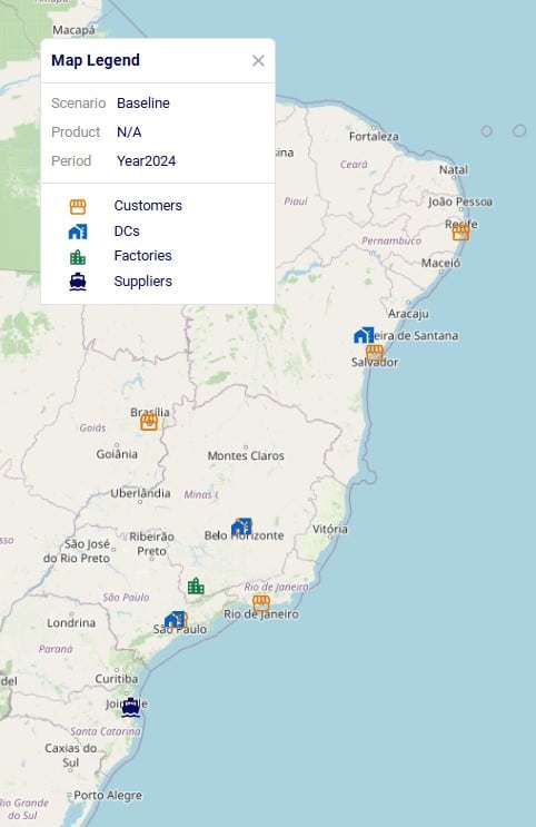
In this example model, 2 products are included: Prod_National to represent products that are made within Brazil at the MK_PousoAlegre_MG factory and Prod_Imported to represent products that are imported, which is supplied from SUP_Itajai_SC within the model, representing the seaport where imported products would arrive. There are 6 customer locations which are in the biggest cities in Brazil; their names start with CLI_. There are also 3 distribution centers (DCs): DC_Barueri_SP, DC_Contagem_MG, and DC_FeiraDeSantana_BA. Note that the 2 letter postfixes in the location names are the abbreviations of the states these locations are in. Please see the next screenshot where all model locations are shown on a map of Brazil:
The model’s horizon is all of 2024 and the 6 customers each have demand for both products, ranging from 100 to 600 units. The SUP_ location (for Prod_Imported) and MK_ location (for Prod_National) replenish the DCs with the products. Between the DCs, some transfers are allowed too. The demand at the customer locations can be fulfilled by 1, 2 or all 3 DCs, depending on the customer. The next screenshot of the Transportation Policies table (filtered for Prod_National) shows which procurement, replenishment, and customer fulfillment flows are allowed:
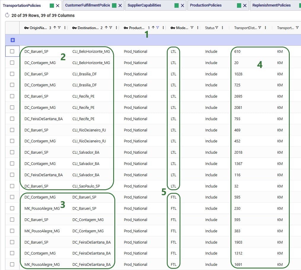
For the other product modelled, Prod_Imported, the same customer fulfillment, DC-DC transfer, and supply options are available, except:
In Brazil, the ICMS tax (Imposto sobre Circulaçao de Mercadorias e Serviços, or Tax on Commerce and Services) is levied by the states. It applies to movement of goods, transportation services between several states or municipalities, and telecommunication services. The rate varies and depends on the state and product.
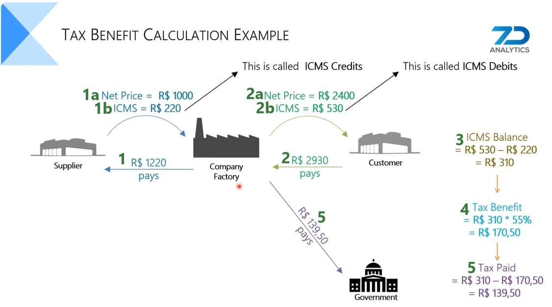
When a company sells a product, the sales price includes ICMS, which results in an ICMS debit for the company (the company owes this to the state). Likewise, when purchasing or transferring product, the ICMS is included in what the company pays the supplier. This creates ICMS credit for the company. The difference between the ICMS debits and credits is what the company will pay as ICMS tax.
The next diagram shows an ICMS tax calculation example, where company also has a 55% tax benefit which is a discount on the ICMS it needs to pay.
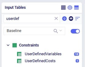
In order to include ICMS tax benefits in a model, we need to be able to calculate ICMS debits and credits based on the amount of flow between locations in different states for both national and imported products. As different states and different products can have different ICMS rates, we need to define these individual flow lanes as variables and apply the appropriate rate to each. This can be done by utilizing the User Defined Variables and User Defined Costs input tables, which can be found in the “Constraints” section of the Cosmic Frog input tables, shown in the below screenshot (here user entered a search term of “userdef” to filter out these 2 tables):
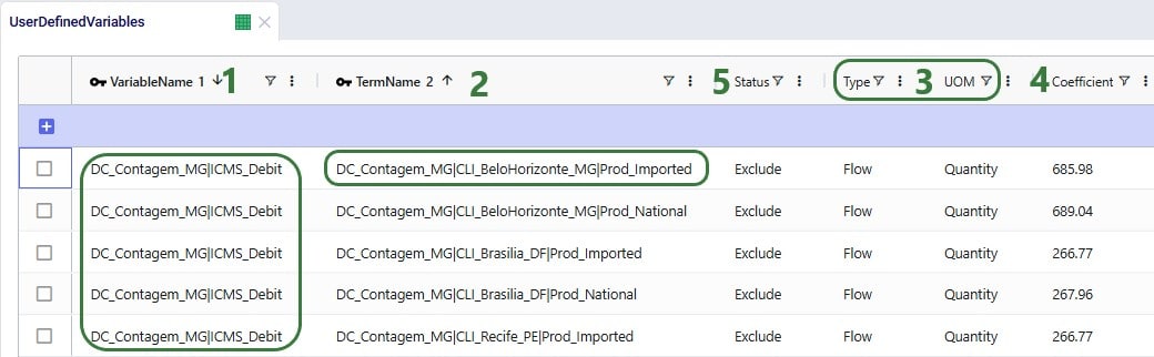
In the User Defined Variables table, we will define 3 variables related to DC_Contagem_MG: one that represents the ICMS Debits, one that represents the ICMS Credits, and one that represents the ICMS Balance (= ICMS Debits – ICMS Credits) for this DC. The ICMS Debits and ICMS Credits variables have multiple terms that each represents a flow out of or a flow into the Contagem DC, respectively. Let us first look at the ICMS Debits variable:
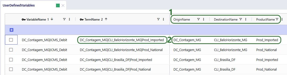
Still looking at the same top records that define the DC_Contagem_MG|ICMS_Debit variable, but freezing the Variable Name and Term Name columns and scrolling right, we can see more of the columns in the User Defined Variables table:
Note that there are quite a few custom columns in this table (not shown in the screenshots; can be added through Grid > Table > Create Custom Column), which were used to calculate the ICMS rates outside of the model. These are helpful to keep in the model, should changes need to be made to the calculations.
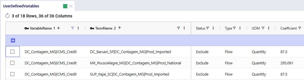
Next, we will have a look at the ICMS Credit variable, which is made up of 3 terms, where each term represents a possible supply/replenishment flow into the Contagem DC:
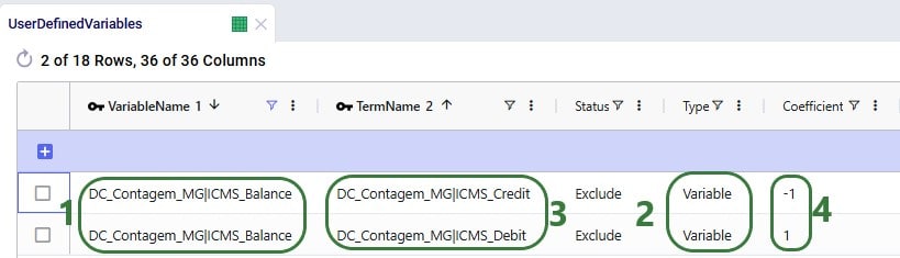
The last step on the User Defined Variables table is to combine the ICMS Credit and ICMS Debit variables to calculate the ICMS balance:
To finalize the setup, we need to add 1 record to the User Defined Costs table, where we will specify that the company has a 55% discount (tax incentive) for the ICMS it pays relating to the Contagem DC:

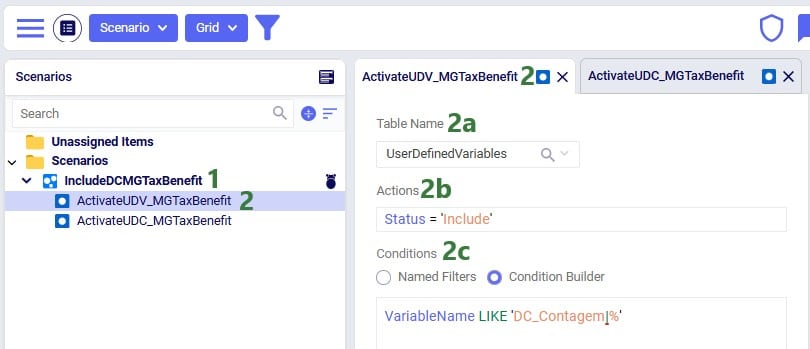
As mentioned in the previous section, all records in the User Defined Variables and User Defined Costs tables have their Status set to Exclude. This way, when the Baseline scenario is run, the ICMS tax incentive is not included, and the network will be optimized just based on the costs included in the model (in this case only transportation costs). We want to include the ICMS tax incentive in a scenario and then compare the outputs with the Baseline scenario. This “IncludeDCMGTaxBenefit” scenario is set up as follows:
Next, we have a look at the second scenario item that is part of this scenario:

With the scenario set up, we run a network optimization (using the Neo engine) on both scenarios and then first look in the Optimization Network Summary output table:
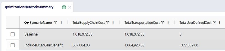
Notice that the Baseline scenario as expected only contains transportation costs, while the IncludeDCMGTaxBenefits scenario also contains user defined costs, which represent the calculated ICMS tax benefit and have a negative value. So, overall, the IncludeDCMGTaxBenefit scenario has about R$ 331k lower total cost as compared to the Baseline scenario, even though the transportation costs are close to R$ 47k higher. Since the transportation costs are different between the 2 scenarios, we expect some of the flows have changed.
There are 3 network optimization output tables that contain the outputs related to User Defined Variables and Costs:

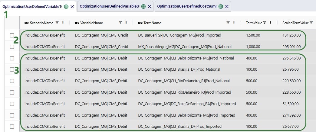
We will first discuss the Optimization User Defined Variable Term Summary output table:
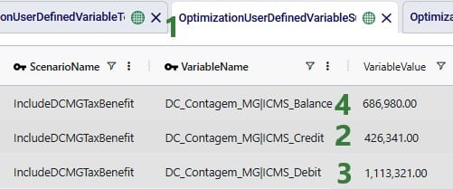
The Optimization User Defined Variable Summary output table contains the outputs at the variable level (e.g. the individual terms of the variables have been aggregated):
Finally, the Optimization User Defined Cost Summary output table shows the cost based on the 55% benefit that was set:
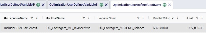
The DC_Contagem_MG_TaxIncentive benefit is calculated from the DC_Contagem_MG|ICMS_Balance variable, where the Variable Value of R$ 686,980 is multiplied by -0.55 to arrive at the Cost value of R$ -377,839.
Now that we understand at a high level the cost impact of the ICMS tax incentive and the details of how this was calculated, let us look at more granular outputs, starting with looking at the flows between locations. Navigate to the Maps module within Cosmic Frog and open the maps named Baseline and Include DC MG Tax Benefit, which show outputs from the Baseline and IncludeDCMGTaxBenefit scenarios, respectively. The next 2 screenshots show the flows from DCs to customer locations: Baseline flows in the top screenshot and scenario “Include DC MG Tax Benefit” flows in the bottom screenshot:
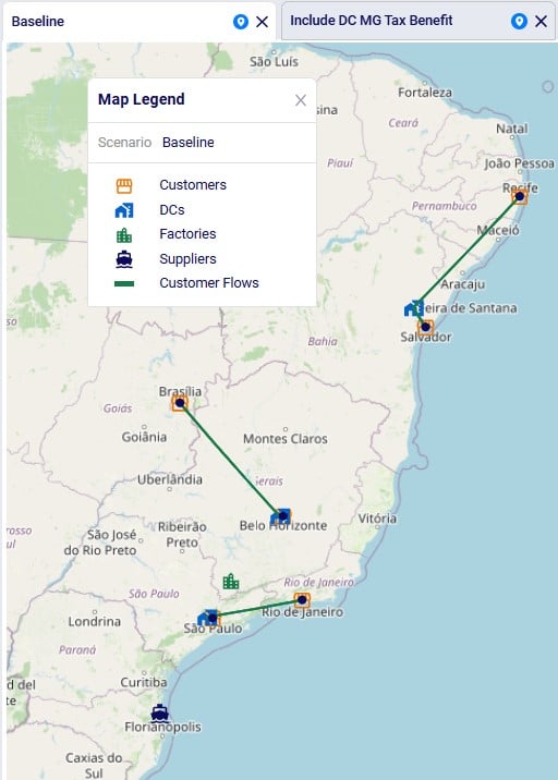
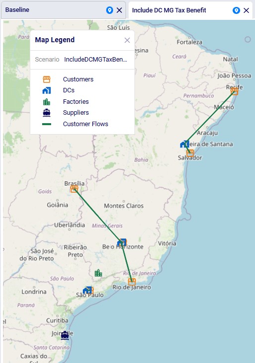
We see that in the Baseline the customer in Rio de Janeiro is served by the DC in Sao Paulo. This changes in the scenario where the tax benefit is included: now the Rio de Janeiro customer is served by the Contagem DC (located close to Belo Horizonte). The other customer fulfillment flows are the same between the 2 scenarios.
This model also has 2 custom dashboards set up in the Analytics module; the 1. Scenarios Overview dashboard contains 2 graphs:

This Summary graph shows the cost buckets for each scenario as a bar chart. As discussed when looking at the Optimization Network Summary output table, the IncludeDCMGTaxBenefit scenario has an overall lower cost due to the tax benefit, which offsets the increased transportation costs as compared to the Baseline scenario.
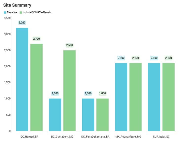
This Site Summary bar chart shows the total outbound quantity for each DC / Factory / Supplier by scenario. We see that the outbound flow for the DC in Barueri is reduced by 500 units in the IncludeDCMGTaxBenefit scenario as compared to the Baseline scenario, whereas the Contagem DC has an increased outbound flow, from 1,000 to 2,500 units. We can examine these shifts in further detail in the second custom dashboard named 2. Outbound Flows by Site, as shown in the next 2 screenshots:

This first screenshot of the dashboard shows the amount of flow from the 3 DCs and the factory to the 6 customer locations. As we already noticed on the map, the only shift here is that the Rio De Janeiro customer is served by the Barueri DC in the Baseline scenario and this changes to it being served by the Contagem DC in the IncludeDCMGTaxBenefit scenario.

Scrolling further right in this table, we see the replenishment flows from the 3 DCs and the Factory to the 3 DCs. There are some more changes here where we see that the flow from the factory to the Barueri DC is reduced by 500 units in the scenario, whereas the flow from the factory to the Contagem DC is increased by 500 units. In the Baseline, the Barueri DC transferred a total of 1,000 units to the other 2 DCs (500 each to the Contagem and Feira de Santana DCs), and the other 2 DCs did not make DC transfers. In the Tax Benefit scenario, the Barueri DC only transfers to the Contagem DC, but now for 1,500 units. We also see that the Contagem DC now transfers 500 units to the Feira de Santana DC, whereas it did not make any transfers in the Baseline scenario.
We hope this gives you a good idea of how taxes and tax incentives can be considered in Cosmic Frog models. Give it a go and let us know of any feedback and/or questions!

Tax systems can be complex, like for example those in Greece, Colombia, Italy, Turkey, and Brazil are considered to be among the most complex ones. It can however be important to include taxes, whether as a cost or benefit or both, in supply chain modeling as they can have a big impact on sourcing decisions and therefore overall costs. Here we will showcase an example of how Cosmic Frog’s User Defined Variables and User Defined Costs can be used to model Brazilian ICMS tax benefits and take these into account when optimizing a supply chain.
The model that is covered in this documentation is the “Brazil Tax Model Example” which was put together by Optilogic’s partner 7D Analytics. It can be downloaded from the the Resource Library. Besides the Cosmic Frog model, the Resource Library content also links to this “Cosmic Frog – BR Tax Model Video” which was also put together by 7D Analytics.
A helpful additional resource for those unfamiliar with Cosmic Frog’s user defined variables, costs, and constraints is this “How to use user defined variables” help article.
In this documentation the setup of the example model will first be briefly explained. Next, the ICMS tax in Brazil will be discussed at a high level, including a simplified example calculation. In the third section, we will cover how ICMS tax benefits can be modelled in Cosmic Frog. And finally, we will look at the impact of including these ICMS tax benefits on the flows and overall network costs.
One quick note upfront is that the screenshots of Cosmic Frog tables used throughout this help article may look different when comparing to the same model in user’s account after taking it from the Resource Library. This is due to columns having been moved or hidden and grids being filtered/sorted in specific ways to show only the most relevant information in these screenshots.
In this example model, 2 products are included: Prod_National to represent products that are made within Brazil at the MK_PousoAlegre_MG factory and Prod_Imported to represent products that are imported, which is supplied from SUP_Itajai_SC within the model, representing the seaport where imported products would arrive. There are 6 customer locations which are in the biggest cities in Brazil; their names start with CLI_. There are also 3 distribution centers (DCs): DC_Barueri_SP, DC_Contagem_MG, and DC_FeiraDeSantana_BA. Note that the 2 letter postfixes in the location names are the abbreviations of the states these locations are in. Please see the next screenshot where all model locations are shown on a map of Brazil:
The model’s horizon is all of 2024 and the 6 customers each have demand for both products, ranging from 100 to 600 units. The SUP_ location (for Prod_Imported) and MK_ location (for Prod_National) replenish the DCs with the products. Between the DCs, some transfers are allowed too. The demand at the customer locations can be fulfilled by 1, 2 or all 3 DCs, depending on the customer. The next screenshot of the Transportation Policies table (filtered for Prod_National) shows which procurement, replenishment, and customer fulfillment flows are allowed:
For the other product modelled, Prod_Imported, the same customer fulfillment, DC-DC transfer, and supply options are available, except:
In Brazil, the ICMS tax (Imposto sobre Circulaçao de Mercadorias e Serviços, or Tax on Commerce and Services) is levied by the states. It applies to movement of goods, transportation services between several states or municipalities, and telecommunication services. The rate varies and depends on the state and product.
When a company sells a product, the sales price includes ICMS, which results in an ICMS debit for the company (the company owes this to the state). Likewise, when purchasing or transferring product, the ICMS is included in what the company pays the supplier. This creates ICMS credit for the company. The difference between the ICMS debits and credits is what the company will pay as ICMS tax.
The next diagram shows an ICMS tax calculation example, where company also has a 55% tax benefit which is a discount on the ICMS it needs to pay.
In order to include ICMS tax benefits in a model, we need to be able to calculate ICMS debits and credits based on the amount of flow between locations in different states for both national and imported products. As different states and different products can have different ICMS rates, we need to define these individual flow lanes as variables and apply the appropriate rate to each. This can be done by utilizing the User Defined Variables and User Defined Costs input tables, which can be found in the “Constraints” section of the Cosmic Frog input tables, shown in the below screenshot (here user entered a search term of “userdef” to filter out these 2 tables):
In the User Defined Variables table, we will define 3 variables related to DC_Contagem_MG: one that represents the ICMS Debits, one that represents the ICMS Credits, and one that represents the ICMS Balance (= ICMS Debits – ICMS Credits) for this DC. The ICMS Debits and ICMS Credits variables have multiple terms that each represents a flow out of or a flow into the Contagem DC, respectively. Let us first look at the ICMS Debits variable:
Still looking at the same top records that define the DC_Contagem_MG|ICMS_Debit variable, but freezing the Variable Name and Term Name columns and scrolling right, we can see more of the columns in the User Defined Variables table:
Note that there are quite a few custom columns in this table (not shown in the screenshots; can be added through Grid > Table > Create Custom Column), which were used to calculate the ICMS rates outside of the model. These are helpful to keep in the model, should changes need to be made to the calculations.
Next, we will have a look at the ICMS Credit variable, which is made up of 3 terms, where each term represents a possible supply/replenishment flow into the Contagem DC:
The last step on the User Defined Variables table is to combine the ICMS Credit and ICMS Debit variables to calculate the ICMS balance:
To finalize the setup, we need to add 1 record to the User Defined Costs table, where we will specify that the company has a 55% discount (tax incentive) for the ICMS it pays relating to the Contagem DC:
As mentioned in the previous section, all records in the User Defined Variables and User Defined Costs tables have their Status set to Exclude. This way, when the Baseline scenario is run, the ICMS tax incentive is not included, and the network will be optimized just based on the costs included in the model (in this case only transportation costs). We want to include the ICMS tax incentive in a scenario and then compare the outputs with the Baseline scenario. This “IncludeDCMGTaxBenefit” scenario is set up as follows:
Next, we have a look at the second scenario item that is part of this scenario:
With the scenario set up, we run a network optimization (using the Neo engine) on both scenarios and then first look in the Optimization Network Summary output table:
Notice that the Baseline scenario as expected only contains transportation costs, while the IncludeDCMGTaxBenefits scenario also contains user defined costs, which represent the calculated ICMS tax benefit and have a negative value. So, overall, the IncludeDCMGTaxBenefit scenario has about R$ 331k lower total cost as compared to the Baseline scenario, even though the transportation costs are close to R$ 47k higher. Since the transportation costs are different between the 2 scenarios, we expect some of the flows have changed.
There are 3 network optimization output tables that contain the outputs related to User Defined Variables and Costs:
We will first discuss the Optimization User Defined Variable Term Summary output table:
The Optimization User Defined Variable Summary output table contains the outputs at the variable level (e.g. the individual terms of the variables have been aggregated):
Finally, the Optimization User Defined Cost Summary output table shows the cost based on the 55% benefit that was set:
The DC_Contagem_MG_TaxIncentive benefit is calculated from the DC_Contagem_MG|ICMS_Balance variable, where the Variable Value of R$ 686,980 is multiplied by -0.55 to arrive at the Cost value of R$ -377,839.
Now that we understand at a high level the cost impact of the ICMS tax incentive and the details of how this was calculated, let us look at more granular outputs, starting with looking at the flows between locations. Navigate to the Maps module within Cosmic Frog and open the maps named Baseline and Include DC MG Tax Benefit, which show outputs from the Baseline and IncludeDCMGTaxBenefit scenarios, respectively. The next 2 screenshots show the flows from DCs to customer locations: Baseline flows in the top screenshot and scenario “Include DC MG Tax Benefit” flows in the bottom screenshot:
We see that in the Baseline the customer in Rio de Janeiro is served by the DC in Sao Paulo. This changes in the scenario where the tax benefit is included: now the Rio de Janeiro customer is served by the Contagem DC (located close to Belo Horizonte). The other customer fulfillment flows are the same between the 2 scenarios.
This model also has 2 custom dashboards set up in the Analytics module; the 1. Scenarios Overview dashboard contains 2 graphs:
This Summary graph shows the cost buckets for each scenario as a bar chart. As discussed when looking at the Optimization Network Summary output table, the IncludeDCMGTaxBenefit scenario has an overall lower cost due to the tax benefit, which offsets the increased transportation costs as compared to the Baseline scenario.
This Site Summary bar chart shows the total outbound quantity for each DC / Factory / Supplier by scenario. We see that the outbound flow for the DC in Barueri is reduced by 500 units in the IncludeDCMGTaxBenefit scenario as compared to the Baseline scenario, whereas the Contagem DC has an increased outbound flow, from 1,000 to 2,500 units. We can examine these shifts in further detail in the second custom dashboard named 2. Outbound Flows by Site, as shown in the next 2 screenshots:
This first screenshot of the dashboard shows the amount of flow from the 3 DCs and the factory to the 6 customer locations. As we already noticed on the map, the only shift here is that the Rio De Janeiro customer is served by the Barueri DC in the Baseline scenario and this changes to it being served by the Contagem DC in the IncludeDCMGTaxBenefit scenario.
Scrolling further right in this table, we see the replenishment flows from the 3 DCs and the Factory to the 3 DCs. There are some more changes here where we see that the flow from the factory to the Barueri DC is reduced by 500 units in the scenario, whereas the flow from the factory to the Contagem DC is increased by 500 units. In the Baseline, the Barueri DC transferred a total of 1,000 units to the other 2 DCs (500 each to the Contagem and Feira de Santana DCs), and the other 2 DCs did not make DC transfers. In the Tax Benefit scenario, the Barueri DC only transfers to the Contagem DC, but now for 1,500 units. We also see that the Contagem DC now transfers 500 units to the Feira de Santana DC, whereas it did not make any transfers in the Baseline scenario.
We hope this gives you a good idea of how taxes and tax incentives can be considered in Cosmic Frog models. Give it a go and let us know of any feedback and/or questions!