Capacity Expansion enables Cosmic Frog’s network optimization engine (Neo) to determine when, where, and how much additional capacity should be added across your supply chain while optimizing the entire network. It helps answer questions such as:
Instead of manually deciding where capacity should be increased, you can define the available expansion options and their associated costs. During optimization, Neo evaluates whether expanding capacity is economically beneficial compared to other alternatives, such as using existing facilities, opening new facilities, adding new production lines, changing transportation flows, or accepting unmet demand.
Capacity Expansion can be modeled for:
This video briefly explains the Capacity Expansion feature and walks through a life-size example model:
This model is also covered in the Capacity Expansion Example Model section further below, which includes a deeper dive into outputs and additional sensitivity analysis scenarios around demand.
If you just want to get going with Capacity Expansion as quick as possible, follow these steps:
Supply chain networks do not remain static. Demand changes, product mixes shift, and manufacturing or distribution requirements can move between regions. As a result, capacity that is sufficient today may not be sufficient in future periods.
Without Capacity Expansion, future capacity is typically modeled by manually creating scenarios with different fixed capacity levels. This can require significant effort and may overlook lower-cost alternatives.
Capacity Expansion lets Neo consider additional capacity as an optimization decision. You define the expansion options and their associated costs, and Neo determines whether an expansion is justified as part of the overall network solution.
This allows capacity decisions to be evaluated together with sourcing, production, inventory, transportation, and facility decisions rather than in isolation.
Use Capacity Expansion when additional capacity is a possible investment and you want Neo to determine whether, when, and how much capacity should be added.
The following are common situations where Capacity Expansion may be appropriate:
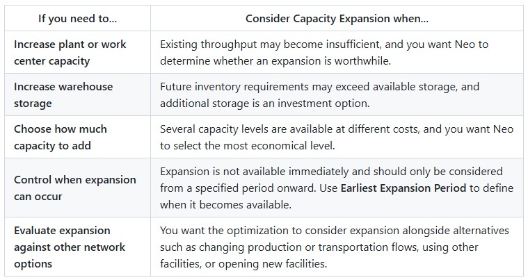
Capacity Expansion can be modeled for facility throughput capacity, facility storage capacity, work center throughput capacity, and user-defined variables.
Rule of thumb question:Is additional capacity an option that Neo should decide on, rather than a change that I have already decided will happen?
Capacity Expansion uses two input tables:
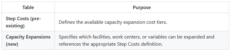
The optimization process is:
Defining Expansion Costs
Capacity Expansion uses the Step Costs table to define available expansion levels and their associated costs.
Each Step Costs definition contains one or more capacity thresholds and the cost associated with reaching that threshold.
During optimization, Neo evaluates these cost tiers and selects the option that minimizes overall network cost.
For example:
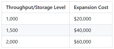
This set of capacity threshold and associated expansion cost steps specifies that:
Rather than requiring the modeler to choose which tier to use, Neo automatically determines whether purchasing additional capacity at what level most reduces the total network cost.
The above tier structure for throughput/storage level and associated expansion cost is entered into the Step Costs table as follows:
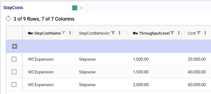
The columns from left to right:
Capacity Expansions Input Table
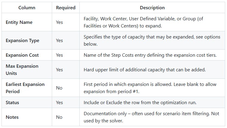
The Capacity Expansions input table associates the throughput/storage level - expansion cost tiers specified in the Step Costs table with the correct entities. Additionally, the type of expansion, the maximum capacity limit, and from when expansion is allowed are configured here too.
Each row in the table represents one entity whose capacity may be expanded.
Expansion Types
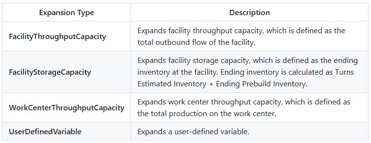
The Expansion Type column supports the following values.
Using the WCExpansion capacity – expansion cost tiers set up in the Step Costs table above, a record that allows a Work Center to expand can look as follows in the Capacity Expansions table:
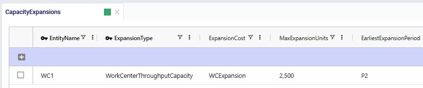
The columns from left to right:
After optimization, the selected capacity expansion decisions are written to the Optimization Capacity Expansion Summary output table.
Each row represents the expansion details of one entity for one scenario-period combination.
Key output fields include:
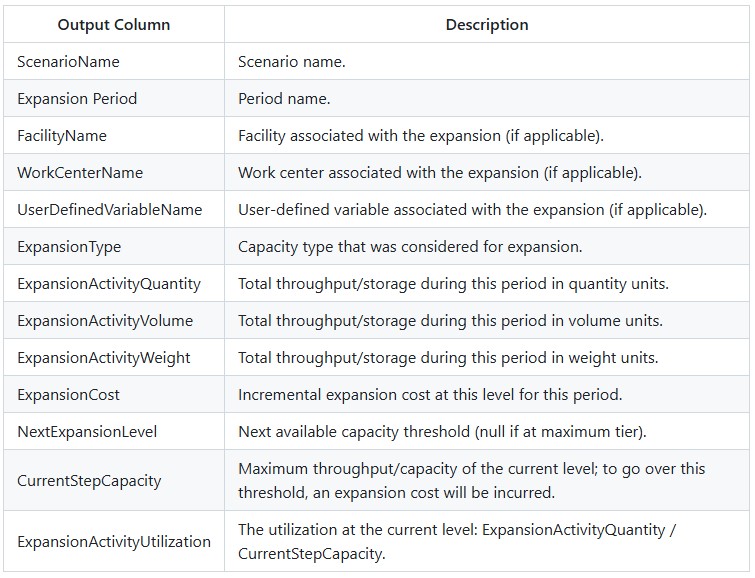
Example output for scenario using above capacity-cost structure to allow WC1 to expand:
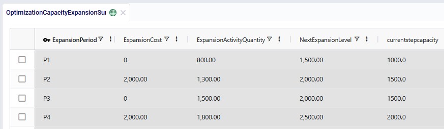
The Scenario Name, Work Center Name (WC1), and Expansion Type (Work Center Throughput Capacity) columns are omitted in this screenshot as they have the same value for all 4 records. The other columns from left to right are:
No additional model option is required.
If the Capacity Expansions table contains one or more rows with Status = Include, Capacity Expansion is automatically considered during optimization.
The Expansion Cost column references a Step Costs entry by name. If the referenced Step Costs entry does not exist, preprocessing will fail.
Max Expansion Units represents a hard upper limit.
If the model requires more capacity than this limit allows, demand may need to be satisfied using other network alternatives or the model may become infeasible.
Because expansion costs are one-time investments, the Neo engine may apply an expansion earlier than expected if there is no incentive to delay it. To ensure expansions occur as late as possible, introduce costs that discourage early investment. For example:
To quickly see which entities are expanded when, use a Greater Than filter with value of 0 in the Expansion Cost field on the Optimization Capacity Expansion Summary table. This resulting grid only shows records where an expansion occurred.
Capacity Expansion and Incremental Change can both be used to model how a network evolves over time, but they solve different problems.
Capacity Expansion gives Neo the option to add capacity and lets the optimization determine whether, when, where, and how much capacity to add, based on the available expansion options and their costs.
Incremental Change controls the pace and sequence of network changes over time. It is designed to make a transition between network states more practical by limiting how much certain types of change can occur from one period to the next. The Incremental Change Constraints table defines the change type and the change budget for each period.
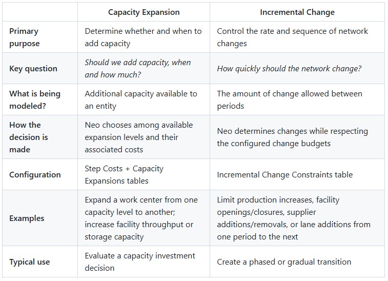
For example, suppose demand is expected to increase, and a work center may eventually need more capacity. Capacity Expansion can allow Neo to decide whether the work center should be expanded, and which expansion level is most economical.
If the resulting network also needs to be implemented gradually—for example, production cannot increase too quickly from one period to the next—Incremental Change can be used to constrain the rate of that transition. Incremental Change currently supports changes such as facilities opened or closed, suppliers added or removed, production increases or decreases, and lanes added.
In short:
Capacity Expansion determines the capacity investment decision; Incremental Change controls how quickly the network can transition.
The two capabilities therefore address different aspects of network evolution and are useful together when both the capacity decision and the pace of implementation need to be modeled.
This example model shows how Capacity Expansion can be used to determine whether the current supply chain network has sufficient capacity to support projected demand from 2027 through 2031 and, if not, to identify the most appropriate and cost-effective capacity expansion strategy. Using several scenarios, the model determines:
Sensitivity analysis around demand growth is performed on the best-looking scenario.
This example model, “Capacity Expansion”, can be copied from the Resource Library if you want to follow along: Capacity Expansion resource.
The Capacity Expansion model is derived from the Global Supply Chain Strategy model from the Resource Library (here) and has been modified to demonstrate Capacity Expansion functionality.
Materials flow through the network as follows:
The model also includes potential West Coast expansion locations:
These facilities are evaluated in selected scenarios.
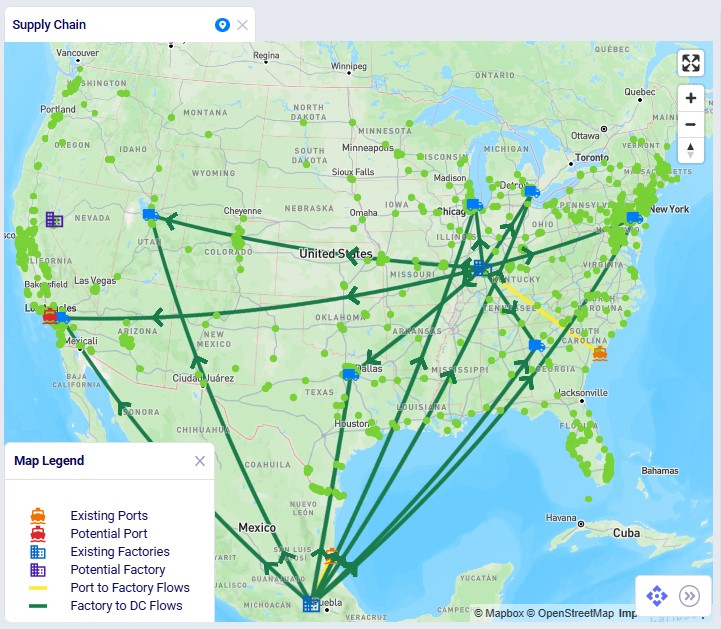
The following map screenshot shows the port, factory, DC, and customer locations in North America, with the current (2026) port to factory and factory to DC flows drawn:
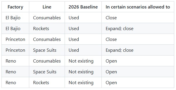
The 9 raw materials are brought into the factories and turned into 3 finished goods on product-specific production lines (Work Centers). Bills of materials are used to specify how much of each raw material is used to produce a unit of a finished good. The following table summarizes current and future production options:
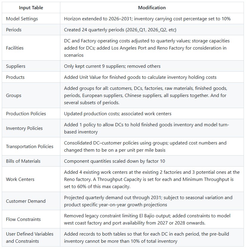
Several changes were made to the base model to support the capacity expansion options and the consideration of the West Coast locations:
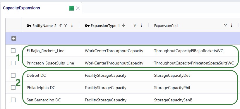
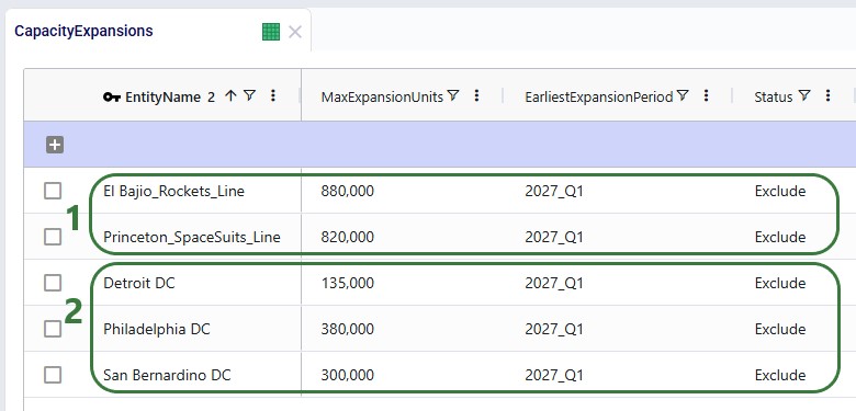
In addition, the Step Costs and Capacity Expansions tables are populated in order to model the possible DC Storage Capacity and Work Center Throughput Capacity expansions in several scenarios. These are discussed in more detail in the next 2 sections.
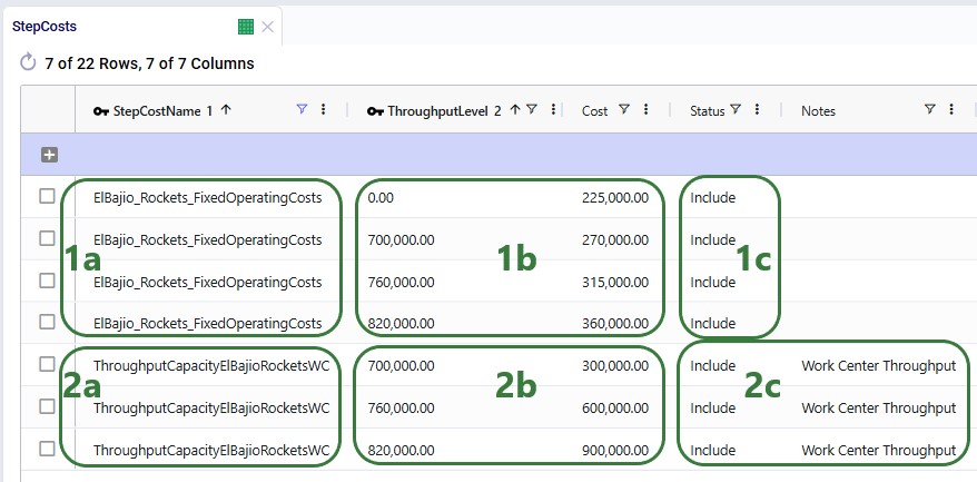
The Step Costs table contains several sets of records with following step cost names:
This screenshot shows the configuration of the Fixed Operating Costs and Expansion Costs of the Rockets line at the El Bajio factory:
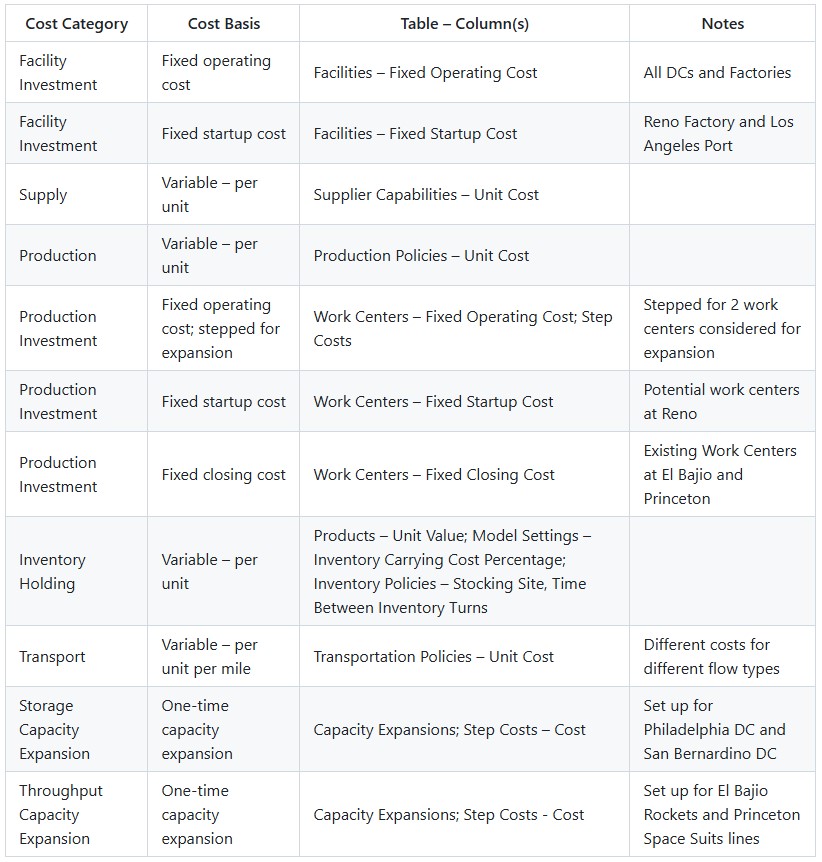
The table below summarizes the different costs that are included in the model:
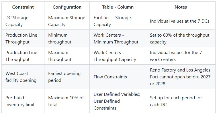
Following table provides an overview of the constraints used in the model:
The objective of the scenario analysis is to determine whether the current supply chain network has sufficient capacity to support projected demand from 2027 through 2031 and, if not, to identify the most appropriate and cost-effective capacity expansion strategy.
The analysis follows a progressive scenario-building approach. Each scenario builds on the findings of the previous scenario(s), allowing the capacity requirements and potential expansion strategies to be evaluated step by step.
The overall storyline is:
1. Test the current network against future demand
The current network (0 Baseline 2026 scenario) is tested against projected 2027–2031 demand. The resulting 0 Baseline 2026-2031 scenario is infeasible, confirming that additional capacity is required.
2. Identify where capacity is insufficient
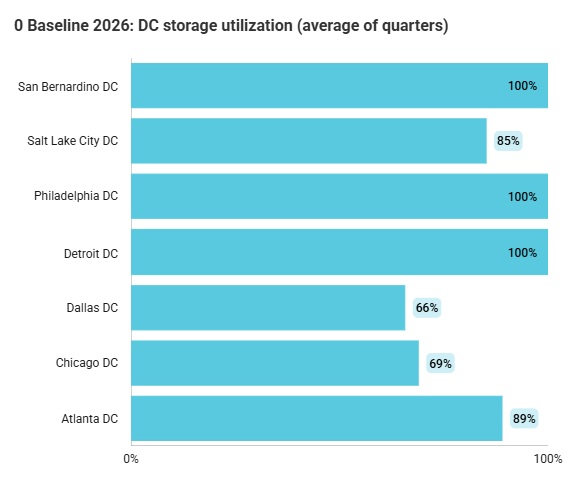
An Infeasibility Check and analysis of outputs of the 0 Baseline 2026 scenario identifies the main constraints. Three DCs — Detroit, Philadelphia, and San Bernardino — are consistently at maximum storage capacity, while two production lines show high utilization: Rockets at El Bajio and Space Suits at Princeton.
3. Address the distribution capacity constraints
Based on these findings, storage capacity at Detroit, Philadelphia, and San Bernardino is allowed to expand and this option is carried forward into all subsequent scenarios.
4. Evaluate alternative production capacity strategies
Two main approaches are compared:
Different Reno start dates (from 2027, scenario 2a, and from 2028, scenario 2b) are also tested to understand the impact of factory startup lead-time.
5. Select the preferred production strategy
The initial comparison shows that **Reno available from 2027 (**scenario 2a) has the lowest cost of the individual alternatives tested. The combined strategy of **Reno from 2027 plus existing-line expansion (**scenario 3) then produces a further, albeit small, cost improvement.
6. Take the combined strategy forward
Scenario 3 Consider Reno from 2027 PLUS Existing Line Expansion is therefore selected as the preferred configuration for further analysis.
7. Test the robustness of the preferred solution
Finally, sensitivity scenarios 4a–4d test how the preferred network configuration performs when demand differs from the forecast by −10%, −5%, +5%, and +10%.
Overall conclusion
The analysis therefore moves from:
“Is the current network sufficient?”
to:
“Where are the capacity constraints?”
to:
“What capacity expansion strategy provides the best solution?”
and finally, to:
“Is the preferred solution robust if demand differs from the forecast?”
The detailed sections that follow below provide the scenario results, screenshots, capacity constraints, cost comparisons, and sensitivity results supporting each step of this decision process.
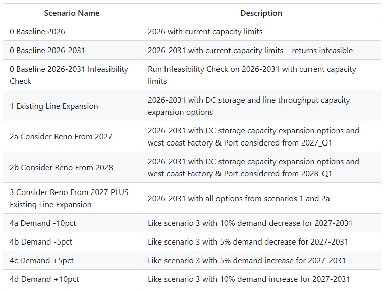
This table summarizes the scenarios:
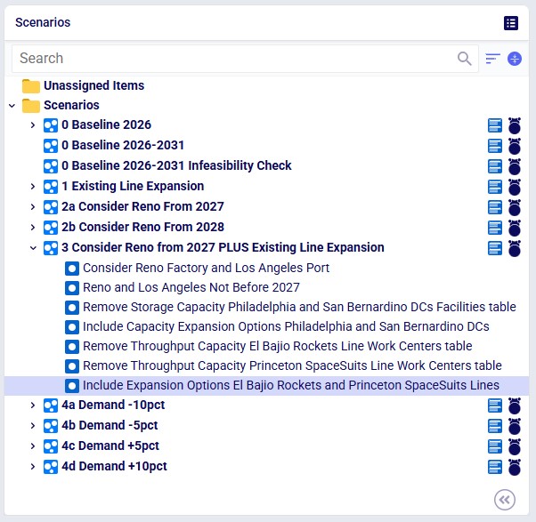
The Scenarios module in the Capacity Expansion model in Cosmic Frog looks as follows. Scenario 3 is expanded, and its 7 scenario items are shown:
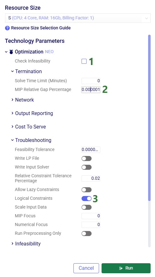
When running scenarios, on the Run Settings modal we need to pay attention to 3 parameters:
Scenario: 0 Baseline 2026
This scenario represents the current supply chain network and capacity configuration and provides the baseline for the analysis.
The key question is:
“Can the current network support the projected demand for 2027–2031 without additional capacity?”
To answer this, projected demand for 2027–2031 was applied to the existing network.
Result
The resulting scenario, 0 Baseline 2026-2031, is infeasible.
This indicates that the existing network does not have sufficient capacity to meet the projected demand throughout the 2027–2031 planning horizon.
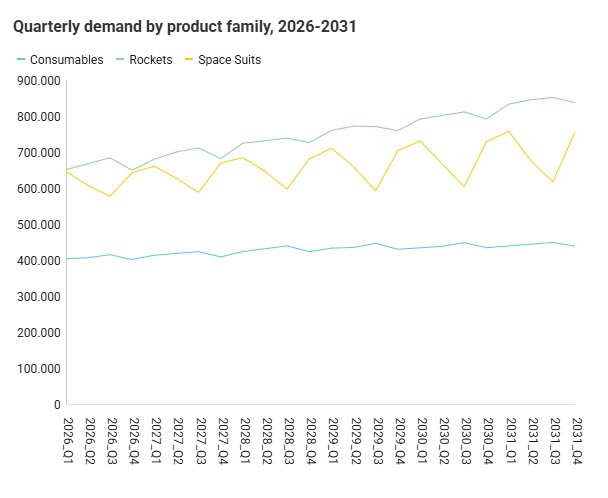
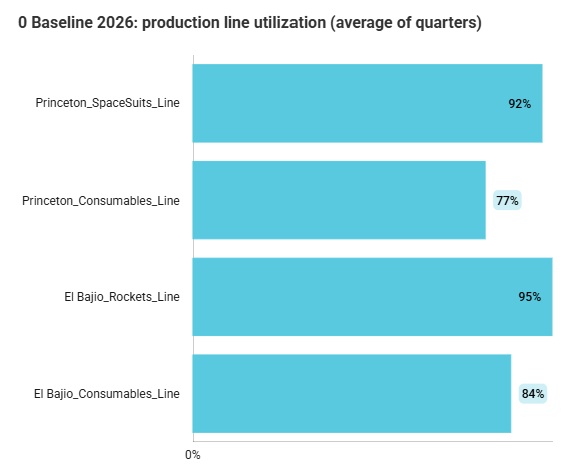
See the “Capacity Story 1 – 2026 Capacity” dashboard in the Analytics module which looks at scenarios 0 Baseline 2026 and 0 Baseline 2026-2031. At the top the overall demand, existing line capacity and the 2026 Baseline total cost are summarized. Beneath these statistics is a table summarizing the 2 scenarios in terms of solve status, total cost, and total demand units served.
Four charts then follow:
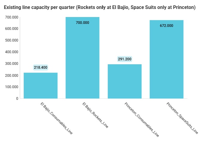
We can for example already calculate that the total Rockets capacity will not be sufficient to meet the demand:
Scenario: 0 Baseline 2026-2031 Infeasibility Check
An Infeasibility Check was performed on a copy of the 2027–2031 baseline scenario to identify which capacity constraints are driving the infeasibility. And just above we have seen where capacity is at a high utilization already during 2026.
See the “Capacity Story 2 – Capacity Shortages 2027-2031” dashboard in the Analytics module. At the top are 2 maps showing DC storage capacity utilization and work center throughput capacity utilization by location in the 0 Baseline 2026 scenario. This shows the same data as the last 2 charts of the first dashboard discussed above, but now on a map.
The next chart in the dashboard shows the extra capacity that would be needed by quarter. For DCs this means additional storage capacity and for factories additional production line capacity:
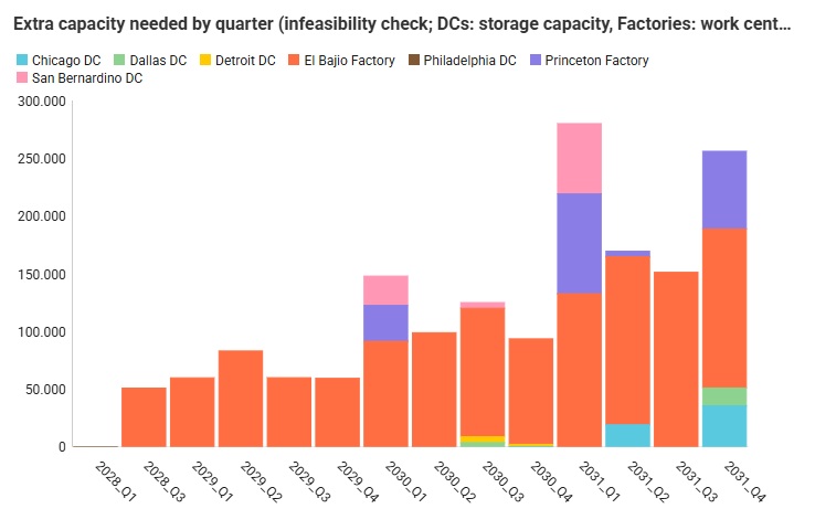
To get a sense for how much additional capacity is needed as compared to what is available today, the following chart showing the peak shortfall as compared to the capacity limit is part of the dashboard too:
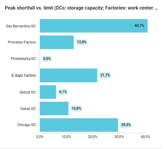
The details of what capacity had to berelaxed when and by how much are also included on a table at the bottom of thedashboard:
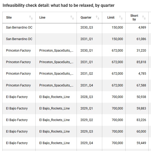
In summary, the analysis identified two main areas of concern:
1. Distribution capacity
Three Distribution Centers (DCs) consistently operate at their maximum storage capacity across all quarters:
Decision:
Storage capacity at these three DCs is allowed to expand in all subsequent scenarios.
2. Production capacity
Two production lines also show high utilization:
These constraints indicate that additional production capacity may be required, and at this point two strategic alternatives will be considered:
Option 1: Expand Existing Production Lines
Scenario: 1 Existing Line Expansion
This scenario addresses the production constraint by allowing the two existing lines with high utilization to expand:
No new factory is introduced.
Option 2: Add a New Factory in Reno
A second strategy is to introduce a new factory in Reno, capable of producing all three products.
Because a new factory requires a start-up lead time, two scenarios are evaluated:
Scenario: 2a Consider Reno From 2027
Reno is available from Q1 2027.
This represents an optimistic assumption in which the new factory can be operational from the beginning of the planning horizon.
Scenario: 2b Consider Reno From 2028
Reno becomes available from Q1 2028.
This represents the more realistic timing assumption based on the expected lead time required to establish the new factory.
In the outputs (the Optimization Facility Summary output table), we see that the Reno Factory opens as soon as it is allowed to in both the 2a and 2b scenario (2027 Q1 and 2028 Q1, respectively).
The total cost of the three scenarios is ranked as follows, see the Optimization Network Summary output table:
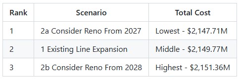
The results show that bringing Reno online from 2027 produces the lowest cost among the initial production capacity alternatives.
Although opening Reno in 2028 is operationally more realistic, its later availability results in a higher overall cost.
Decision:
The analysis proceeds with the assumption that Reno should be considered as available from Q1 2027 in the subsequent scenarios.
Scenario: 3 Consider Reno from 2027 PLUS Existing Line Expansion
The next question is whether the optimal strategy is to combine both approaches:
Result
The combined strategy produces a slightly lower overall cost of $2,147.42M than 2a Consider Reno From 2027, which was previously the lowest-cost scenario:
This indicates that combining new capacity in Reno with targeted expansion of the existing production lines provides a better overall network solution than relying on Reno alone.
Decision
Scenario 3 is therefore selected as the preferred scenario for further sensitivity analysis.
See the “Capacity Story 3 – Expand and Add Capacity 2027-2031” dashboard in the Analytics module for more high-level details of scenarios 1, 2a, 2b, and 3. At the top, a table and 2 charts summarize the scenarios by total costs and by cost type.
The next chart and table focus on capacity expansion costs and timing:
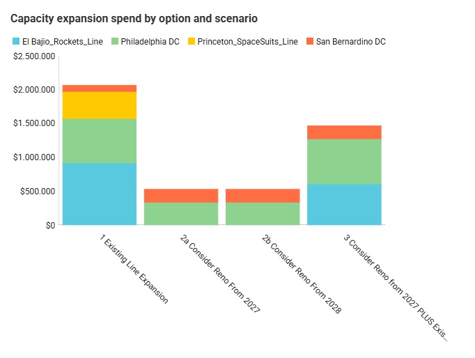
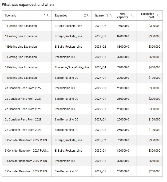
Three more charts on this dashboard show production by quarter: by factory comparing scenarios 1 and 3, and for scenario 3 also a chart that shows throughput for the new Reno production lines.
First, we will look at different charts and output tables to see when and where expansions occur, next summarize these in a table, and finally explain the expansion decisions.
The example model contains a dashboard named “Capacity Expansion – Expansion Costs by Scenario and Period” in the Analytics module. It contains 2 charts:
The “Total Expansion Cost by Scenario” chart for scenarios 1, 2a, 2b, and 3 looks as follows:
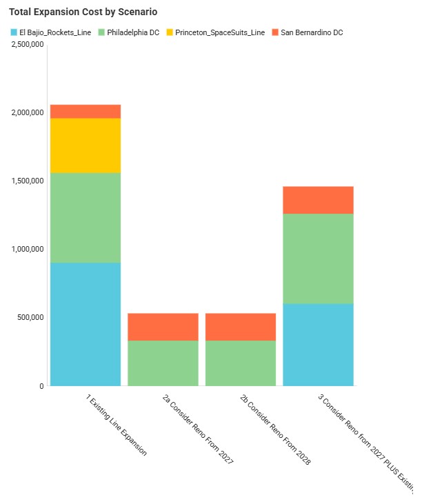
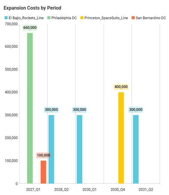
To drill into period-specific details, we use the “Expansion Costs by Period” chart, here filtered for scenario 1:
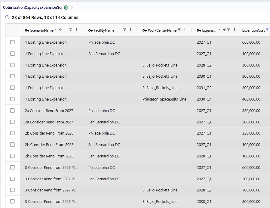
We can also see these details for all scenarios in table form in the Optimization Capacity Expansion Summary output table, which is filtered for Expansion Cost > 0 here:
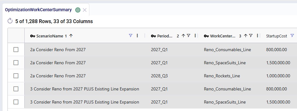
To get the full picture, we also check if any existing lines close, and if so when. In addition, we can check if all 3 potential production lines at Reno are being used and, if so, from the first possible option (2027_Q1) or later. This screenshot filters the Optimization Work Center Summary output table for scenarios 2a and 3 and Startup Cost > 0:
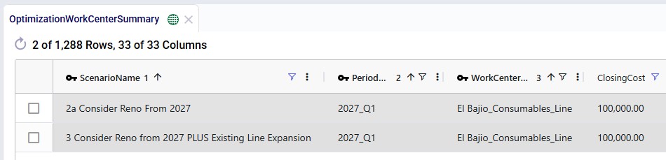
And here is the Optimization Work Center Summary output table again, still filtered for scenarios 2a and 3, but now also for Closing Cost > 0:
For storage capacity expansion at the DCs, in all 4 scenarios (1, 2a, 2b, and 3):
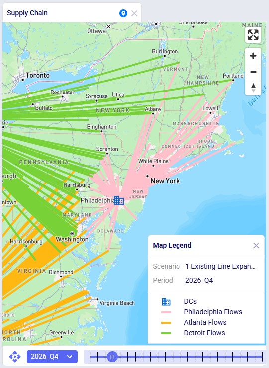
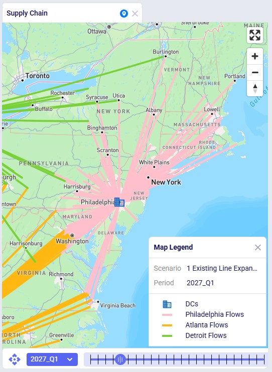
Next, we will focus on scenarios 1, 2a, and 3 as we have seen 2a is preferred over 2b and explain the drivers behind the differences in expansions. We will start with a summary of the scenarios and their results:
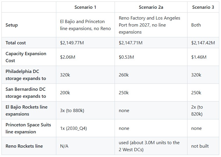
Why San Bernardino expands to 250k in scenarios 2a and 3
The Reno Factory opens in scenarios 2a and 3 and due to its proximity, San Bernardino services a lot more customer demand since the overall cost is reduced due to the much lower inbound costs. Note that in scenario 3, Rockets do still come from the El Bajio Factory.
Why Philadelphia expands to 320k in scenarios 1 and 3 and to 260k in scenario 2a
Philadelphia’s upgrade costs an extra $330k to go from 260k to 320k. How much it saves differs by scenario:
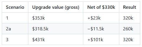
Why El Bajio Rockets expands three times in scenario 1 and twice in scenario 3
Rockets all come from El Bajio in both. Scenario 3 builds about 60k extra Rockets ahead in each of periods 2030_Q3 through 2031_Q1 (about 220k unit-quarters of pre-build, vs about 41k in scenario 1), while scenario 1 buys the 880k step for 2031_Q2.
Scenario 3 can do this because it has 50k more storage, all at San Bernardino, which pulls customers from Dallas and Salt Lake City and frees room there.
Why Princeton Space Suits expands in scenario 1 and not in 2a and 3
Scenario 1 does not have any other options to add Space Suits production capacity, so it needs to expand the existing line at the Princeton Factory to meet the increasing demand. The Space Suits line in Reno is opened as soon as Reno opens in 2027_Q1 in scenarios 2a and 3. This provides sufficient capacity for Space Suits over the model's horizon so that additional investment for expansion of the existing Space Suits line at the Princeton Factory is not needed.
Scenarios: 4a–4d
The preferred configuration is tested against different demand assumptions to determine how sensitive the solution is to changes in the 2027–2031 demand forecast.
Four demand scenarios are evaluated:
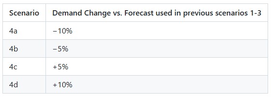
The purpose of this analysis is to understand whether the preferred capacity strategy remains appropriate if actual demand is lower or higher than currently forecast.
On the Optimization Network Summary Output table, we see that, as expected, the total supply chain cost is lowest for the lowest demand scenario (4a), and it increases as demand increases:
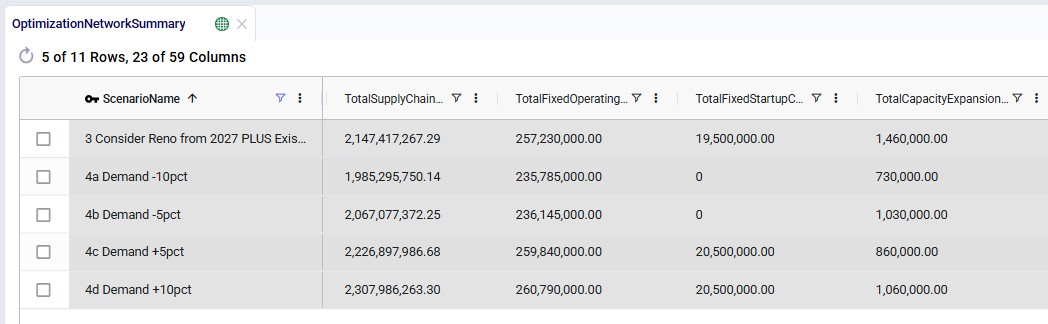
Most other costs are omitted here, but from the Total Fixed Operating and Total Fixed Startup costs, we can tell that the Reno Factory and Los Angeles Port do not come online in the scenarios with reduced demand (4a and 4b), but they do in those with higher demand (4c and 4d).
Now we will compare how the expansion costs are split out over the DCs and existing lines in these 5 scenarios by using the Total Expansion Cost by Scenario chart in the Analytics module:
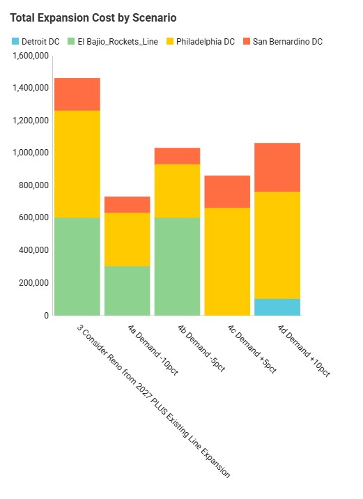
For the timing of each expansion, we can again use the Optimization Capacity Expansion Summary output table, now filtered for Expansion Cost > 0 and scenarios 3 and 4a-d:
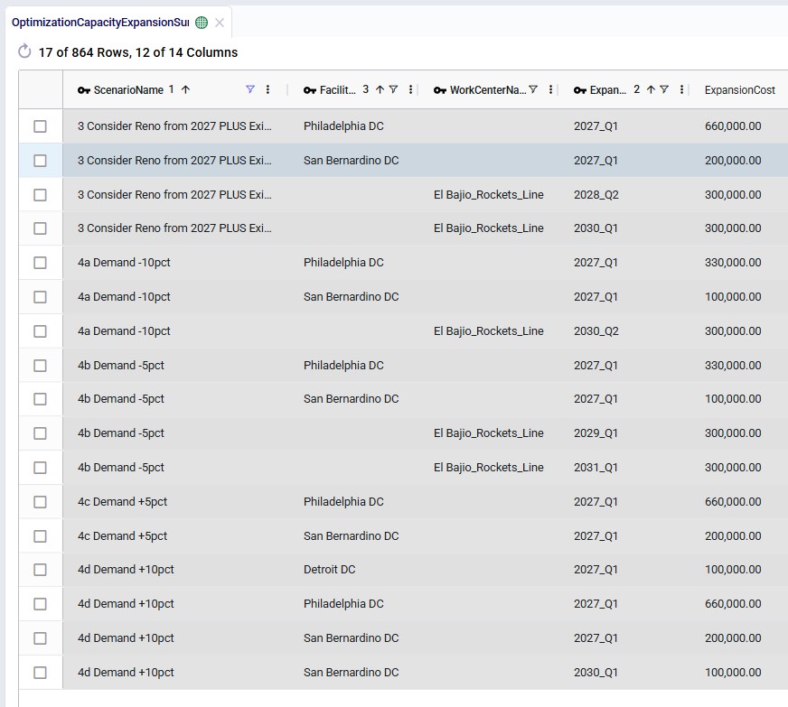
For scenarios 4a-d, we can then conclude:
The following Help Center articles cover several modeling concepts touched upon in this article in more detail:
And to get started with Optilogic tools, please see the following documentation landing pages for:
The following SQL statements can be used to add and (re-)populate a custom column named custom_entityname to the Optimization Capacity Expansion Summary output table. This was done in the example model using the SQL Editor application to enable several visuals in the Capacity Expansion specific dashboards showing different types of expansions together in one chart.
The ALTER TABLE statement can be used once for a model to add the column and then does not need to be used again. The example model already has this column, so no need to run it on that model. The UPDATE statement needs to be run after running any new scenarios and after re-running already existing scenarios.
ALTER TABLE anura_2_8.optimizationcapacityexpansionsummary
  ADD COLUMN custom_entityname text;

UPDATE anura_2_8.optimizationcapacityexpansionsummary SET custom_entityname = COALESCE(
  NULLIF(BTRIM(facilityname), ''),
  NULLIF(BTRIM(workcentername), ''),
  NULLIF(BTRIM(userdefinedvariablename), '')
);
Note that you could also achieve this by using Ada with following prompts that has the Cosmic Frog model selected as the database and using the Modeler Agent:

Capacity Expansion enables Cosmic Frog’s network optimization engine (Neo) to determine when, where, and how much additional capacity should be added across your supply chain while optimizing the entire network. It helps answer questions such as:
Instead of manually deciding where capacity should be increased, you can define the available expansion options and their associated costs. During optimization, Neo evaluates whether expanding capacity is economically beneficial compared to other alternatives, such as using existing facilities, opening new facilities, adding new production lines, changing transportation flows, or accepting unmet demand.
Capacity Expansion can be modeled for:
This video briefly explains the Capacity Expansion feature and walks through a life-size example model:
This model is also covered in the Capacity Expansion Example Model section further below, which includes a deeper dive into outputs and additional sensitivity analysis scenarios around demand.
If you just want to get going with Capacity Expansion as quick as possible, follow these steps:
Supply chain networks do not remain static. Demand changes, product mixes shift, and manufacturing or distribution requirements can move between regions. As a result, capacity that is sufficient today may not be sufficient in future periods.
Without Capacity Expansion, future capacity is typically modeled by manually creating scenarios with different fixed capacity levels. This can require significant effort and may overlook lower-cost alternatives.
Capacity Expansion lets Neo consider additional capacity as an optimization decision. You define the expansion options and their associated costs, and Neo determines whether an expansion is justified as part of the overall network solution.
This allows capacity decisions to be evaluated together with sourcing, production, inventory, transportation, and facility decisions rather than in isolation.
Use Capacity Expansion when additional capacity is a possible investment and you want Neo to determine whether, when, and how much capacity should be added.
The following are common situations where Capacity Expansion may be appropriate:
Capacity Expansion can be modeled for facility throughput capacity, facility storage capacity, work center throughput capacity, and user-defined variables.
Rule of thumb question:Is additional capacity an option that Neo should decide on, rather than a change that I have already decided will happen?
Capacity Expansion uses two input tables:
The optimization process is:
Defining Expansion Costs
Capacity Expansion uses the Step Costs table to define available expansion levels and their associated costs.
Each Step Costs definition contains one or more capacity thresholds and the cost associated with reaching that threshold.
During optimization, Neo evaluates these cost tiers and selects the option that minimizes overall network cost.
For example:
This set of capacity threshold and associated expansion cost steps specifies that:
Rather than requiring the modeler to choose which tier to use, Neo automatically determines whether purchasing additional capacity at what level most reduces the total network cost.
The above tier structure for throughput/storage level and associated expansion cost is entered into the Step Costs table as follows:
The columns from left to right:
Capacity Expansions Input Table
The Capacity Expansions input table associates the throughput/storage level - expansion cost tiers specified in the Step Costs table with the correct entities. Additionally, the type of expansion, the maximum capacity limit, and from when expansion is allowed are configured here too.
Each row in the table represents one entity whose capacity may be expanded.
Expansion Types
The Expansion Type column supports the following values.
Using the WCExpansion capacity – expansion cost tiers set up in the Step Costs table above, a record that allows a Work Center to expand can look as follows in the Capacity Expansions table:
The columns from left to right:
After optimization, the selected capacity expansion decisions are written to the Optimization Capacity Expansion Summary output table.
Each row represents the expansion details of one entity for one scenario-period combination.
Key output fields include:
Example output for scenario using above capacity-cost structure to allow WC1 to expand:
The Scenario Name, Work Center Name (WC1), and Expansion Type (Work Center Throughput Capacity) columns are omitted in this screenshot as they have the same value for all 4 records. The other columns from left to right are:
No additional model option is required.
If the Capacity Expansions table contains one or more rows with Status = Include, Capacity Expansion is automatically considered during optimization.
The Expansion Cost column references a Step Costs entry by name. If the referenced Step Costs entry does not exist, preprocessing will fail.
Max Expansion Units represents a hard upper limit.
If the model requires more capacity than this limit allows, demand may need to be satisfied using other network alternatives or the model may become infeasible.
Because expansion costs are one-time investments, the Neo engine may apply an expansion earlier than expected if there is no incentive to delay it. To ensure expansions occur as late as possible, introduce costs that discourage early investment. For example:
To quickly see which entities are expanded when, use a Greater Than filter with value of 0 in the Expansion Cost field on the Optimization Capacity Expansion Summary table. This resulting grid only shows records where an expansion occurred.
Capacity Expansion and Incremental Change can both be used to model how a network evolves over time, but they solve different problems.
Capacity Expansion gives Neo the option to add capacity and lets the optimization determine whether, when, where, and how much capacity to add, based on the available expansion options and their costs.
Incremental Change controls the pace and sequence of network changes over time. It is designed to make a transition between network states more practical by limiting how much certain types of change can occur from one period to the next. The Incremental Change Constraints table defines the change type and the change budget for each period.
For example, suppose demand is expected to increase, and a work center may eventually need more capacity. Capacity Expansion can allow Neo to decide whether the work center should be expanded, and which expansion level is most economical.
If the resulting network also needs to be implemented gradually—for example, production cannot increase too quickly from one period to the next—Incremental Change can be used to constrain the rate of that transition. Incremental Change currently supports changes such as facilities opened or closed, suppliers added or removed, production increases or decreases, and lanes added.
In short:
Capacity Expansion determines the capacity investment decision; Incremental Change controls how quickly the network can transition.
The two capabilities therefore address different aspects of network evolution and are useful together when both the capacity decision and the pace of implementation need to be modeled.
This example model shows how Capacity Expansion can be used to determine whether the current supply chain network has sufficient capacity to support projected demand from 2027 through 2031 and, if not, to identify the most appropriate and cost-effective capacity expansion strategy. Using several scenarios, the model determines:
Sensitivity analysis around demand growth is performed on the best-looking scenario.
This example model, “Capacity Expansion”, can be copied from the Resource Library if you want to follow along: Capacity Expansion resource.
The Capacity Expansion model is derived from the Global Supply Chain Strategy model from the Resource Library (here) and has been modified to demonstrate Capacity Expansion functionality.
Materials flow through the network as follows:
The model also includes potential West Coast expansion locations:
These facilities are evaluated in selected scenarios.
The following map screenshot shows the port, factory, DC, and customer locations in North America, with the current (2026) port to factory and factory to DC flows drawn:
The 9 raw materials are brought into the factories and turned into 3 finished goods on product-specific production lines (Work Centers). Bills of materials are used to specify how much of each raw material is used to produce a unit of a finished good. The following table summarizes current and future production options:
Several changes were made to the base model to support the capacity expansion options and the consideration of the West Coast locations:
In addition, the Step Costs and Capacity Expansions tables are populated in order to model the possible DC Storage Capacity and Work Center Throughput Capacity expansions in several scenarios. These are discussed in more detail in the next 2 sections.
The Step Costs table contains several sets of records with following step cost names:
This screenshot shows the configuration of the Fixed Operating Costs and Expansion Costs of the Rockets line at the El Bajio factory:
The table below summarizes the different costs that are included in the model:
Following table provides an overview of the constraints used in the model:
The objective of the scenario analysis is to determine whether the current supply chain network has sufficient capacity to support projected demand from 2027 through 2031 and, if not, to identify the most appropriate and cost-effective capacity expansion strategy.
The analysis follows a progressive scenario-building approach. Each scenario builds on the findings of the previous scenario(s), allowing the capacity requirements and potential expansion strategies to be evaluated step by step.
The overall storyline is:
1. Test the current network against future demand
The current network (0 Baseline 2026 scenario) is tested against projected 2027–2031 demand. The resulting 0 Baseline 2026-2031 scenario is infeasible, confirming that additional capacity is required.
2. Identify where capacity is insufficient
An Infeasibility Check and analysis of outputs of the 0 Baseline 2026 scenario identifies the main constraints. Three DCs — Detroit, Philadelphia, and San Bernardino — are consistently at maximum storage capacity, while two production lines show high utilization: Rockets at El Bajio and Space Suits at Princeton.
3. Address the distribution capacity constraints
Based on these findings, storage capacity at Detroit, Philadelphia, and San Bernardino is allowed to expand and this option is carried forward into all subsequent scenarios.
4. Evaluate alternative production capacity strategies
Two main approaches are compared:
Different Reno start dates (from 2027, scenario 2a, and from 2028, scenario 2b) are also tested to understand the impact of factory startup lead-time.
5. Select the preferred production strategy
The initial comparison shows that **Reno available from 2027 (**scenario 2a) has the lowest cost of the individual alternatives tested. The combined strategy of **Reno from 2027 plus existing-line expansion (**scenario 3) then produces a further, albeit small, cost improvement.
6. Take the combined strategy forward
Scenario 3 Consider Reno from 2027 PLUS Existing Line Expansion is therefore selected as the preferred configuration for further analysis.
7. Test the robustness of the preferred solution
Finally, sensitivity scenarios 4a–4d test how the preferred network configuration performs when demand differs from the forecast by −10%, −5%, +5%, and +10%.
Overall conclusion
The analysis therefore moves from:
“Is the current network sufficient?”
to:
“Where are the capacity constraints?”
to:
“What capacity expansion strategy provides the best solution?”
and finally, to:
“Is the preferred solution robust if demand differs from the forecast?”
The detailed sections that follow below provide the scenario results, screenshots, capacity constraints, cost comparisons, and sensitivity results supporting each step of this decision process.
This table summarizes the scenarios:
The Scenarios module in the Capacity Expansion model in Cosmic Frog looks as follows. Scenario 3 is expanded, and its 7 scenario items are shown:
When running scenarios, on the Run Settings modal we need to pay attention to 3 parameters:
Scenario: 0 Baseline 2026
This scenario represents the current supply chain network and capacity configuration and provides the baseline for the analysis.
The key question is:
“Can the current network support the projected demand for 2027–2031 without additional capacity?”
To answer this, projected demand for 2027–2031 was applied to the existing network.
Result
The resulting scenario, 0 Baseline 2026-2031, is infeasible.
This indicates that the existing network does not have sufficient capacity to meet the projected demand throughout the 2027–2031 planning horizon.
See the “Capacity Story 1 – 2026 Capacity” dashboard in the Analytics module which looks at scenarios 0 Baseline 2026 and 0 Baseline 2026-2031. At the top the overall demand, existing line capacity and the 2026 Baseline total cost are summarized. Beneath these statistics is a table summarizing the 2 scenarios in terms of solve status, total cost, and total demand units served.
Four charts then follow:
We can for example already calculate that the total Rockets capacity will not be sufficient to meet the demand:
Scenario: 0 Baseline 2026-2031 Infeasibility Check
An Infeasibility Check was performed on a copy of the 2027–2031 baseline scenario to identify which capacity constraints are driving the infeasibility. And just above we have seen where capacity is at a high utilization already during 2026.
See the “Capacity Story 2 – Capacity Shortages 2027-2031” dashboard in the Analytics module. At the top are 2 maps showing DC storage capacity utilization and work center throughput capacity utilization by location in the 0 Baseline 2026 scenario. This shows the same data as the last 2 charts of the first dashboard discussed above, but now on a map.
The next chart in the dashboard shows the extra capacity that would be needed by quarter. For DCs this means additional storage capacity and for factories additional production line capacity:
To get a sense for how much additional capacity is needed as compared to what is available today, the following chart showing the peak shortfall as compared to the capacity limit is part of the dashboard too:
The details of what capacity had to berelaxed when and by how much are also included on a table at the bottom of thedashboard:
In summary, the analysis identified two main areas of concern:
1. Distribution capacity
Three Distribution Centers (DCs) consistently operate at their maximum storage capacity across all quarters:
Decision:
Storage capacity at these three DCs is allowed to expand in all subsequent scenarios.
2. Production capacity
Two production lines also show high utilization:
These constraints indicate that additional production capacity may be required, and at this point two strategic alternatives will be considered:
Option 1: Expand Existing Production Lines
Scenario: 1 Existing Line Expansion
This scenario addresses the production constraint by allowing the two existing lines with high utilization to expand:
No new factory is introduced.
Option 2: Add a New Factory in Reno
A second strategy is to introduce a new factory in Reno, capable of producing all three products.
Because a new factory requires a start-up lead time, two scenarios are evaluated:
Scenario: 2a Consider Reno From 2027
Reno is available from Q1 2027.
This represents an optimistic assumption in which the new factory can be operational from the beginning of the planning horizon.
Scenario: 2b Consider Reno From 2028
Reno becomes available from Q1 2028.
This represents the more realistic timing assumption based on the expected lead time required to establish the new factory.
In the outputs (the Optimization Facility Summary output table), we see that the Reno Factory opens as soon as it is allowed to in both the 2a and 2b scenario (2027 Q1 and 2028 Q1, respectively).
The total cost of the three scenarios is ranked as follows, see the Optimization Network Summary output table:
The results show that bringing Reno online from 2027 produces the lowest cost among the initial production capacity alternatives.
Although opening Reno in 2028 is operationally more realistic, its later availability results in a higher overall cost.
Decision:
The analysis proceeds with the assumption that Reno should be considered as available from Q1 2027 in the subsequent scenarios.
Scenario: 3 Consider Reno from 2027 PLUS Existing Line Expansion
The next question is whether the optimal strategy is to combine both approaches:
Result
The combined strategy produces a slightly lower overall cost of $2,147.42M than 2a Consider Reno From 2027, which was previously the lowest-cost scenario:
This indicates that combining new capacity in Reno with targeted expansion of the existing production lines provides a better overall network solution than relying on Reno alone.
Decision
Scenario 3 is therefore selected as the preferred scenario for further sensitivity analysis.
See the “Capacity Story 3 – Expand and Add Capacity 2027-2031” dashboard in the Analytics module for more high-level details of scenarios 1, 2a, 2b, and 3. At the top, a table and 2 charts summarize the scenarios by total costs and by cost type.
The next chart and table focus on capacity expansion costs and timing:
Three more charts on this dashboard show production by quarter: by factory comparing scenarios 1 and 3, and for scenario 3 also a chart that shows throughput for the new Reno production lines.
First, we will look at different charts and output tables to see when and where expansions occur, next summarize these in a table, and finally explain the expansion decisions.
The example model contains a dashboard named “Capacity Expansion – Expansion Costs by Scenario and Period” in the Analytics module. It contains 2 charts:
The “Total Expansion Cost by Scenario” chart for scenarios 1, 2a, 2b, and 3 looks as follows:
To drill into period-specific details, we use the “Expansion Costs by Period” chart, here filtered for scenario 1:
We can also see these details for all scenarios in table form in the Optimization Capacity Expansion Summary output table, which is filtered for Expansion Cost > 0 here:
To get the full picture, we also check if any existing lines close, and if so when. In addition, we can check if all 3 potential production lines at Reno are being used and, if so, from the first possible option (2027_Q1) or later. This screenshot filters the Optimization Work Center Summary output table for scenarios 2a and 3 and Startup Cost > 0:
And here is the Optimization Work Center Summary output table again, still filtered for scenarios 2a and 3, but now also for Closing Cost > 0:
For storage capacity expansion at the DCs, in all 4 scenarios (1, 2a, 2b, and 3):
Next, we will focus on scenarios 1, 2a, and 3 as we have seen 2a is preferred over 2b and explain the drivers behind the differences in expansions. We will start with a summary of the scenarios and their results:
Why San Bernardino expands to 250k in scenarios 2a and 3
The Reno Factory opens in scenarios 2a and 3 and due to its proximity, San Bernardino services a lot more customer demand since the overall cost is reduced due to the much lower inbound costs. Note that in scenario 3, Rockets do still come from the El Bajio Factory.
Why Philadelphia expands to 320k in scenarios 1 and 3 and to 260k in scenario 2a
Philadelphia’s upgrade costs an extra $330k to go from 260k to 320k. How much it saves differs by scenario:
Why El Bajio Rockets expands three times in scenario 1 and twice in scenario 3
Rockets all come from El Bajio in both. Scenario 3 builds about 60k extra Rockets ahead in each of periods 2030_Q3 through 2031_Q1 (about 220k unit-quarters of pre-build, vs about 41k in scenario 1), while scenario 1 buys the 880k step for 2031_Q2.
Scenario 3 can do this because it has 50k more storage, all at San Bernardino, which pulls customers from Dallas and Salt Lake City and frees room there.
Why Princeton Space Suits expands in scenario 1 and not in 2a and 3
Scenario 1 does not have any other options to add Space Suits production capacity, so it needs to expand the existing line at the Princeton Factory to meet the increasing demand. The Space Suits line in Reno is opened as soon as Reno opens in 2027_Q1 in scenarios 2a and 3. This provides sufficient capacity for Space Suits over the model's horizon so that additional investment for expansion of the existing Space Suits line at the Princeton Factory is not needed.
Scenarios: 4a–4d
The preferred configuration is tested against different demand assumptions to determine how sensitive the solution is to changes in the 2027–2031 demand forecast.
Four demand scenarios are evaluated:
The purpose of this analysis is to understand whether the preferred capacity strategy remains appropriate if actual demand is lower or higher than currently forecast.
On the Optimization Network Summary Output table, we see that, as expected, the total supply chain cost is lowest for the lowest demand scenario (4a), and it increases as demand increases:
Most other costs are omitted here, but from the Total Fixed Operating and Total Fixed Startup costs, we can tell that the Reno Factory and Los Angeles Port do not come online in the scenarios with reduced demand (4a and 4b), but they do in those with higher demand (4c and 4d).
Now we will compare how the expansion costs are split out over the DCs and existing lines in these 5 scenarios by using the Total Expansion Cost by Scenario chart in the Analytics module:
For the timing of each expansion, we can again use the Optimization Capacity Expansion Summary output table, now filtered for Expansion Cost > 0 and scenarios 3 and 4a-d:
For scenarios 4a-d, we can then conclude:
The following Help Center articles cover several modeling concepts touched upon in this article in more detail:
And to get started with Optilogic tools, please see the following documentation landing pages for:
The following SQL statements can be used to add and (re-)populate a custom column named custom_entityname to the Optimization Capacity Expansion Summary output table. This was done in the example model using the SQL Editor application to enable several visuals in the Capacity Expansion specific dashboards showing different types of expansions together in one chart.
The ALTER TABLE statement can be used once for a model to add the column and then does not need to be used again. The example model already has this column, so no need to run it on that model. The UPDATE statement needs to be run after running any new scenarios and after re-running already existing scenarios.
ALTER TABLE anura_2_8.optimizationcapacityexpansionsummary
  ADD COLUMN custom_entityname text;

UPDATE anura_2_8.optimizationcapacityexpansionsummary SET custom_entityname = COALESCE(
  NULLIF(BTRIM(facilityname), ''),
  NULLIF(BTRIM(workcentername), ''),
  NULLIF(BTRIM(userdefinedvariablename), '')
);
Note that you could also achieve this by using Ada with following prompts that has the Cosmic Frog model selected as the database and using the Modeler Agent: