The use of non alpha-numeric characters can present the possibilities of data issues when running scenarios. The only special characters that will be officially supported are periods, dashes, parentheses and underscores.
Please note that while other special characters in input data or scenario names can still function as expected, we can not guarantee that they will always work. If you encounter any issues or have questions about the data being used, please feel free to contact support at support@optilogic.com.
The Anura data schema enables design in the Optilogic platform. It sits above the design algorithms to create a consistent modeling paradigm for our algorithms:
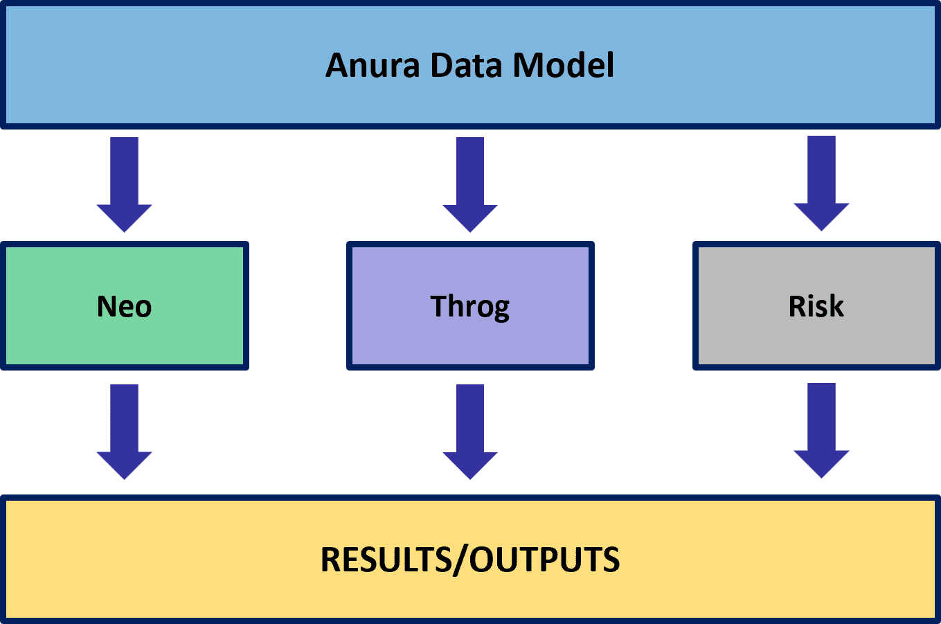
Anura is comprised of modeling categories required to build a model. Each modeling category contains tables to add pertinent detail and/or complexity to your model as well as identify structure, policies, costs, and constraints.
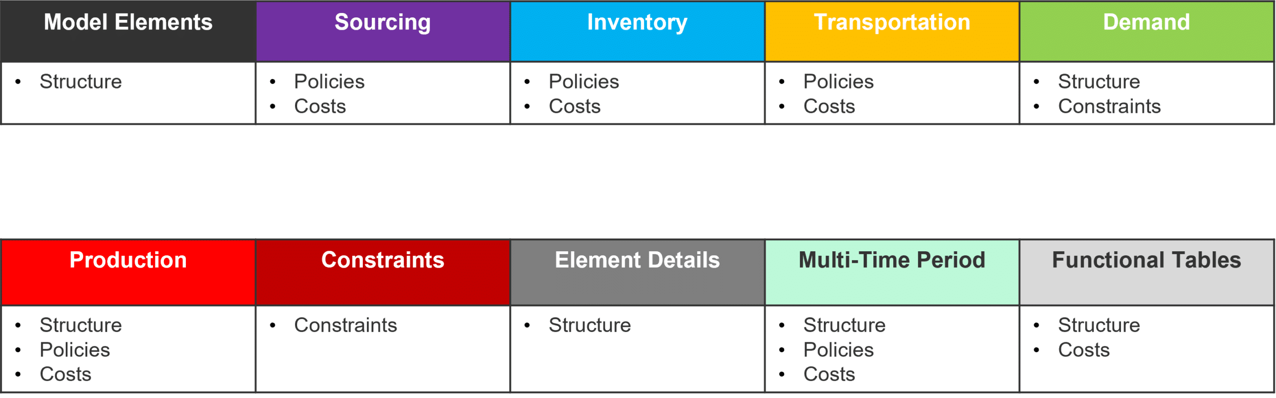
A complete list of the tables and fields within each table can be downloaded locally here.
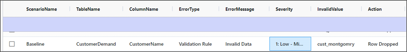
The validation error report table will be populated for all model solves and contains a lot of helpful information for both reviewing and troubleshooting models. A set of results will be saved for each scenario and every record will report the table and column where the issue has been identified, a description of the error, the value that was identified as the problem along with the action taken by the solver. In the instance where multiple records are generated for the same type of error, you will see an example record populated as the identified value and a count of the errors will be displayed – detailed records can be printed using debug mode. Each record will also be rated on the severity of its impact on a scale from 0 – 3 with 3 being the highest.
The validation error report can serve as a great tool to help troubleshoot an infeasible model. The best approach for utilizing this table is to first sort on the Severity column so that the highest level issues are displayed. If severity 3 issues are present, they must be addressed. If no severity 3 issues exist, the next steps would be to review any severity 2 issues to consider policy impact. It is also helpful to search for any instances where rows are being dropped as these dropped rows will likely influence other errors. To do this, filter the Action field for ‘Row Dropped’.
While the report can be helpful in trying to proactively diagnose infeasible models, it won’t always have all of the answers. To learn more about the dedicated engine for infeasibility diagnosis please check out this article: Troubleshooting With The Infeasibility Diagnostic Engine
Severity 3 records capture instances of syntax issues that are preventing the model from being built properly. This can be presented as 2 types:
Severity 3 records can also be instances where model infeasibility can be detected before the model solve begins, in the instance where a severity 3 error is detected the model solve will be cancelled immediately. There are 3 common instances of these Severity 3 errors:
Severity 2 records capture sources of potential infeasibility and while not always a definitive reason for a problem being infeasible, they will highlight potential issues with the policy structure of a model. There are 2 common instances of Severity 2 errors:
These severity 2 errors don’t necessarily indicate a problem, they can often times be caused by grouped-based policies and members overlapping from one group to another. It is still a good idea to review these gaps in policies and make sure that all of the lanes which should be considered in your solve are in fact being read into the solver.
Severity 1 records will capture issues in model data that can cause rows from input tables to be dropped when writing the solver files for a model. These can be issues on allowed numerical ranges, a negative quantity for customer demand as an example. Detailed policy linkages that do not align can also cause errors, for example a process which uses a specific workcenter that doesn’t exist at the assigned facility. There are other causes of severity 1 errors, and it is important to review these errors for any changes that are made to your input data. Be sure to check the Action column to see if a default value was applied and note the new value that was used, or if a row was being dropped.
Severity 1 records will also note other issues that have been identified in the model input data. These can be unused model elements such as a customer which is included but has no demand, or transportation modes that exist in the model but aren’t assigned to any lanes. There can also be records generated for policies that have no cost charged against them to let you know that a cost is missing. Duplicate data records will also be flagged as severity 1 errors – the last row read in by the solver will be persisted. If you have duplicated data with different detailed information these duplicates should be addressed in your input tables so that you can make sure the correct information is read in by the solver.
A point to look out for is any severity 1 issue that is related to an invalid UOM entry – these will cause records to be dropped and while the dropped records don’t always directly cause model infeasibilities themselves, they can often times be at the root of other issues identified as higher severity or through infeasibility diagnosis runs.
Severity 0 records are for informational purposes only and are generated when records have been excluded upstream, either in the input tables directly or by other corrective actions that the solver has taken. These records are letting you know that the solver read in the input records but they did not correspond to anything that was in the current solve. An example of this would be if you only included a subset of your facilities for a scenario, but still had included records for an out-of-scope MFG location. If the MFG is excluded in the facilities table but its production policies are still included, a record will be written to the table to let you know that these production policy rows were skipped.
Utilities enable powerful modelling capabilities for use cases like integration to other services or data sources, repeatable data transformation or anything that can be supported by Python! System Utilities are available as a core capability in Cosmic Frog for use cases like LTL rate lookups, TransitMatrix time & distance generation, and copying items like Maps and Dashboards from one model to another. More useful System Utilities will become available in Cosmic Frog over time. Some of these System Utilities are also available in the Resource Library where they can be downloaded from, and then customized and made available to modelers for specific projects or models. In this Help Article we will cover both how to use use System Utilities as well as how to customize and deploy Custom Utilities.
The “Using and Customizing Utilities” resource in the Resource Library includes a helpful 15-minute video on Cosmic Frog Model Utilities and users are encouraged to watch this.
In this Help Article, System Utilities will be covered first, before discussing the specifics of creating one’s own Utilities. Finally, how to use and share Custom Utilities will be explained as well.
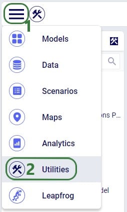
Users can access utilities within Cosmic Frog by going to the Utilities section via the Module Menu drop-down:
Once in the Utilities section, user will see the list of available utilities:
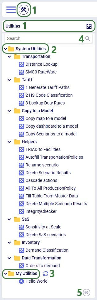
The appendix of this Help Article contains a table of all System Utilities and their descriptions.
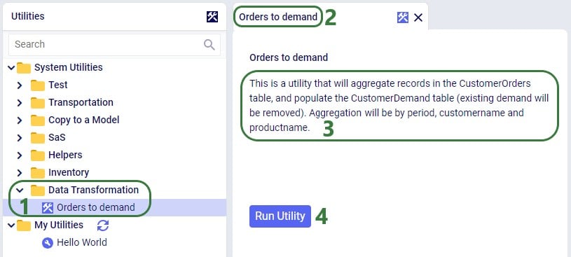
Utilities vary in complexity by how many input parameters a user can configure and range from those where no parameters need to be set at all to those where many can be set. Following screenshot shows the Orders to Demand utility which does not require any input parameters to be set by the user:
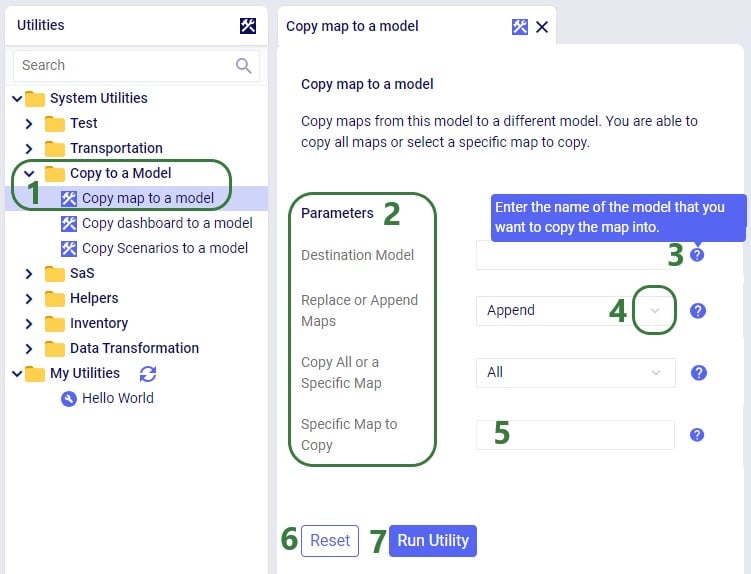
The Copy map to a model utility shown in the next screenshot does require several parameters to be set by the user:
When the Run Utility button has been clicked, a message appears beneath it briefly:
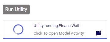
Clicking on this message will open the Model Activity pane to the right of the tab(s) with open utilities:

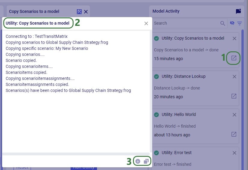
Users will not only see activities related to running utilities in the Model Activity list. Other actions that are executed within Cosmic Frog will be listed here too, like for example when user has geocoded locations by using the Geocode tool on the Customers / Facilities / Suppliers tables or when user makes a change in a master table and chooses to cascade these changes to other tables.
Please note that the following System Utilities have separate Help Articles where they are explained in more detail:
The utilities that are available in the Resource Library can be downloaded by users and then customized to fit the user’s specific needs. Examples are to change the logic of a data transformation, apply similar logic but to a different table, etc. Or users may even build their own utilities entirely. If a user updates a utility or creates a new one, they can share these back with other users so they can benefit from them as well.
Utilities are Python scripts that contain a specific structure which will be explained in this section. They can be edited directly in the Atlas application on the Optilogic platform or users can download the Python file that is being used as a starting point and edit it using an IDE (Integrated Development Environment) installed on their computer. A rich text editor geared towards coding, like for example Visual Studio Code, will work fine too for most. An advantage of working locally is that user can take advantage of code completion features (auto-completion while typing, showing what arguments functions need, catch incorrect syntax/names, etc.) by installing an extension package like for example IntelliSense (for Visual Studio Code). The screenshots of the Python files underlying the utilities that follow in this documentation are taken while working with them in Visual Studio Code locally and on a machine that has the IntelliSense extension package installed.
A great resource on how to write Python scripts for Cosmic Frog models is this “Scripting with Cosmic Frog” video. In this video, the cosmicfrog Python library, which adds specific functionality to the existing Python features to work with Cosmic Frog models, is covered in some detail.
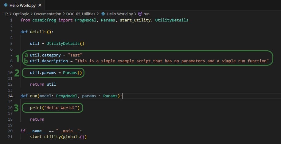
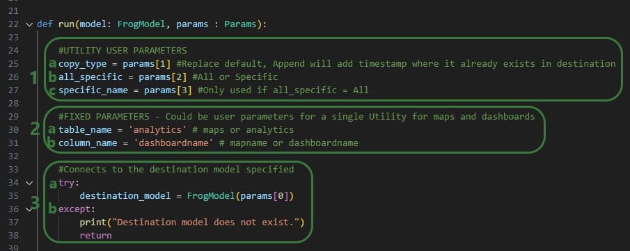
We will start by looking at the Python file of the very simple Hello World utility. In this first screenshot, the parts that can stay the same for all utilities are outlined in green:

Next, onto the parts of the utility’s Python script that users will want to update when customizing / creating their own scripts:
Now, we will discuss how input parameters, which users can then set in Cosmic Frog, can be added to the details function. After that we will cover different actions that can be added to the run function.
If a utility needs to be able to take any inputs from a user before running it, these are created by adding parameters in the details function of the utility’s Python script:

We will take a closer look at a utility that uses parameters and map the arguments of the parameters back to what the user sees when the utility is open in Cosmic Frog, see the next 2 screenshots: the numbers in the script screenshot are matched to those in the Cosmic Frog screenshot to indicate what code leads to what part of the utility when looking at it in Cosmic Frog. These screenshots use the Copy dashboard to a model utility of which the Python script (Copy dashboard to a model.py) was downloaded from the Resource Library.
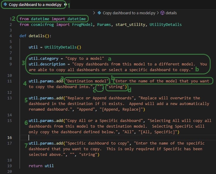
Note that Python lists are 0-indexed, meaning that the first parameter (Destination Model in this example) is referenced by typing params[0], the second parameter (Replace of Append dashboards) by typing params[1], etc. We will see this in the code when adding actions to the run function below too.
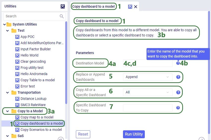
Now let’s have a look at how the above code translates to what a user sees in the Cosmic Frog user interface for the Copy dashboard to a model System Utility (note that the numbers in this screenshot match with those in the above screenshot):
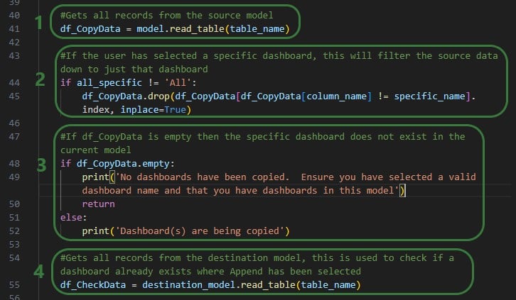
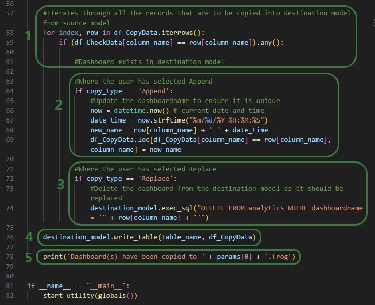
The actions a utility needs to perform are added to the run function of the Python script. These will be different for different types of utilities. We will cover the actions the Copy dashboard to a model utility uses at a high level and refer to Python documentation if user is interested in understanding all the details. There are a lot of helpful resources and communities online where users can learn everything there is to know about using & writing Python code. A great place to start is on the Python for Beginners page on python.org. This page also mentions how more experienced coders can get started with Python. Also note that text in green font that follows a hash sign are comments to add context to code.
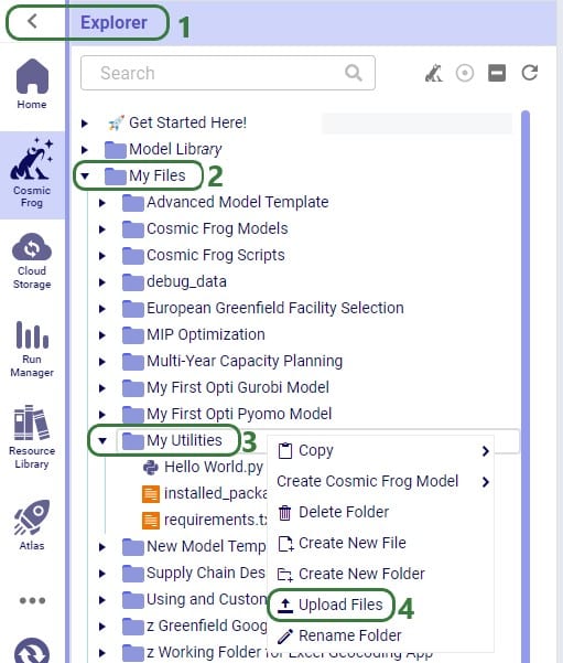
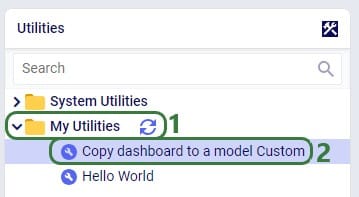
For a custom utility to be showing in the My Utilities category of the utilities list in Cosmic Frog, it needs to be saved under My Files > My Utilities in the user’s Optilogic account:
Note that if a Python utility file is already in user’s Optilogic account, but in a different folder, user can click on it and drag it to the My Utilities folder.
For utilities to work, a requirements.txt file which only contains the text cosmicfrog needs to be placed in the same My Files > My Utilities folder (if not there already):

A customized version of the Copy dashboard to a model utility was uploaded here, and a requirements.txt file is present in the same folder too.
Once a Python utility file is uploaded to My Files > My Utilities, it can be accessed from within Cosmic Frog:
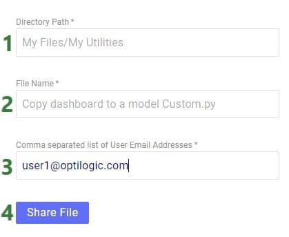
If users want to share custom utilities with other users, they can do so by right-clicking on it and choosing the “Send Copy of File” option:

The following form then opens:
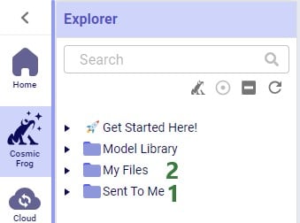
When a custom utility has been shared with you by another user, it will be saved under the Sent To Me folder in your Optilogic account:
Should you have created a custom utility that you feel a lot of other users can benefit from and you are allowed to share outside of your organization, then we encourage you to submit it into Optilogic’s Resource Library. Click on the Contribute button at the left top of the Resource Library and then follow the steps as outlined in the “How can I add Python Modules to the Resource Library?” section towards the end of the “How to use the Resource Library” help article.
Utility names and descriptions by category:
Sequential Objectives allow for you to set multiple tiers of objectives for the optimization solve to consider, where each tier of objectives can be relaxed by a defined percentage when solving for the next tier.
Here is a basic example of how Sequential Objectives can be used.
100 units of demand for P1 at CZ.
Available pathways for flow are as follows:
Find a solution that will first minimize total costs, but then will work to minimize the total amount of travel time in the solution while only relaxing the Total Cost solution by 20%.
When just solving with the standard objective of Profit Maximization, the cheapest path will be utilized. All flows will come from MFG > DC1 > CZ and the total cost will be $500.
We’ve built the Sequential Objectives so that we will first optimize over the Total Supply Chain Cost as Priority 1. We have also set the Tolerance to be 20 which will allow for a 20% relaxation in the solution to solve for the secondary objective – Total Weighted Flow Time.
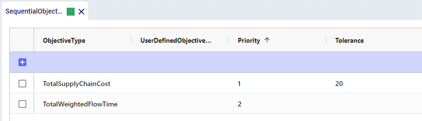
We’ll now see that the more expensive pathway of MFG > DC2 > CZ is used as it requires less travel time. Because the initial cost was $500, we will send as many units as possible through DC2 up until the total cost reaches $600 – a 20% deviation from the initial cost. This results is 5 units flowing via DC2, while 95 units remain through DC1 for a total cost of $600.
This example model can be found in the Resource Library listed under the name of Sequential Objectives Demo.
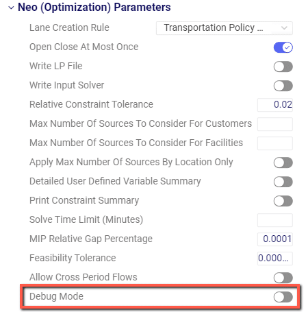
Running a model in debug mode can be a helpful troubleshooting tool as it will print more detailed reports of model issues.
The run option for Debug Mode is not included as a default in models but it can be added via the SQL Editor. Please copy and paste the following SQL query and run it against the model database you wish to add the option to.
Copy SQL Query Here: Add Debug Mode Model Run Option SQL Statement
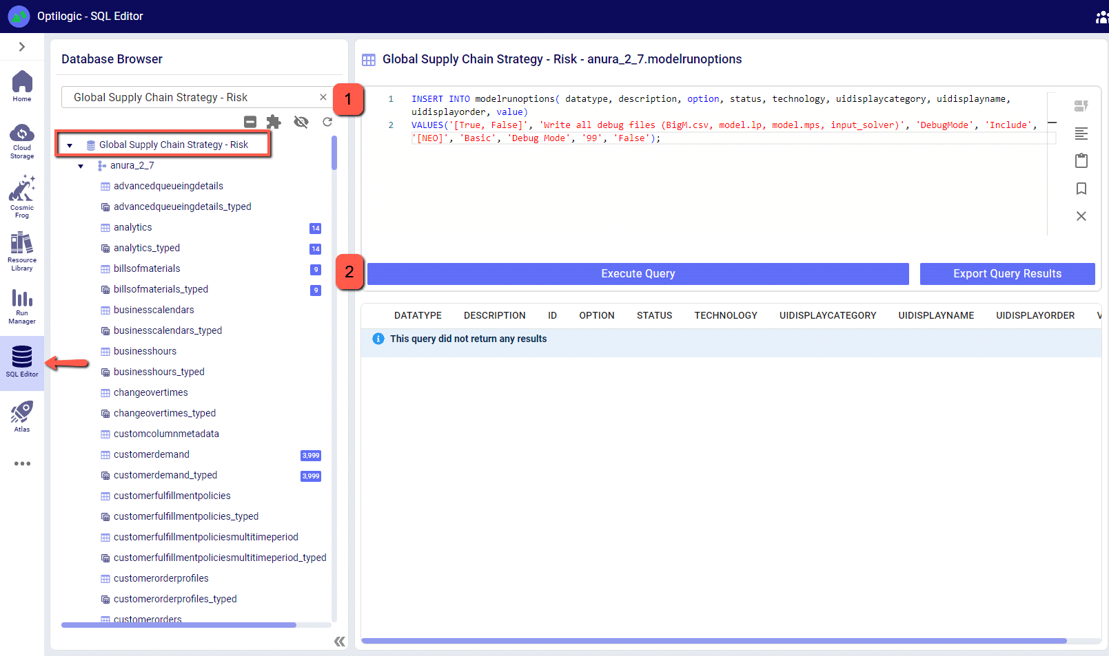
Now, if you open the model again in Cosmic Frog you will see that Debug Mode is an available option in the run screen.
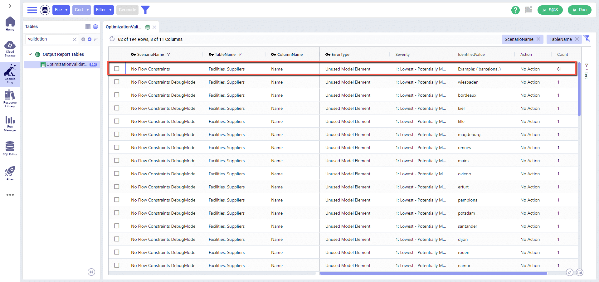
When set to True, Debug Mode will show all instances of validation errors instead of displaying an example of an error and the count of occurrences. You can see the difference in the following screenshot, where 1 row with 61 instances of the same error is turned into 61 individual rows.
Debug Mode will also print and save the input files that are passed to the solver – these will be saved in your File Explorer at My Files > debug_data > ModelName > ScenarioName. For each scenario run with debug mode enabled you will have the following:
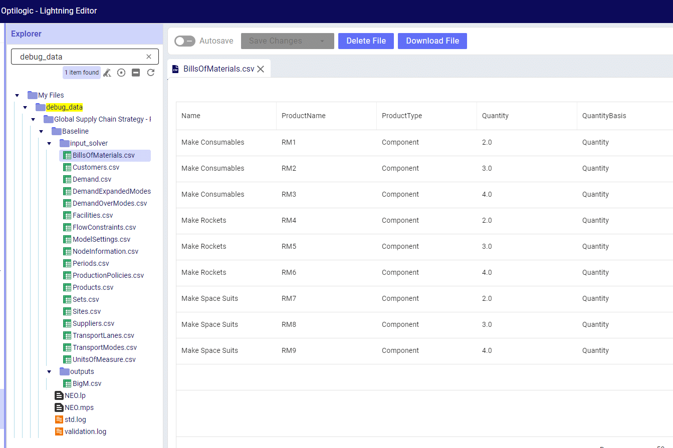
Please note that this data is saved to your File Explorer and for larger models can take up quite a bit of disk space. If you reach 100% disk space utilization you will be unable to run any new jobs as they won’t have any space to write their required data to. The debug_data folder is almost always the cause of this disk space utilization issue, clearing its contents will allow jobs to start again.
If you have any questions or concerns about how this might impact your models, please don’t hesitate to reach out to support@optilogic.com.
The nature of LTL freight rating is complex and multi-faceted. The RateWare® XL LTL rating engine of SMC3 enables customers to manage parcel pricing and LTL rating complexity, for both class and density rates, with comprehensive rating solutions.
Cosmic Frog users that hold a license to the RateWare XL LTL Rating Engine of SMC3 can easily use it within Cosmic Frog to lookup LTL rates and use them in their models. In this documentation we will explain where to find the SMC3 RateWare utility within Cosmic Frog and how to use it. First, we will cover the basic inputs needed in Cosmic Frog models, then how to configure and run the SMC3 RateWare Utility to look up LTL rates, and finally how to add those rates for usage in the model.
Before running the SMC3 RateWare Utility to retrieve LTL rates, we need to set up our model, including the origin-destination pairs for which we want to look up the LTL rates. Here, we will cover the inputs of a basic demo model showing how to use the SMC3 RateWare Utility. Of course, models using this utility may be much more complex in setup as compared to what is shown here.
The next 3 screenshots show:
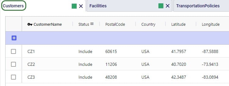
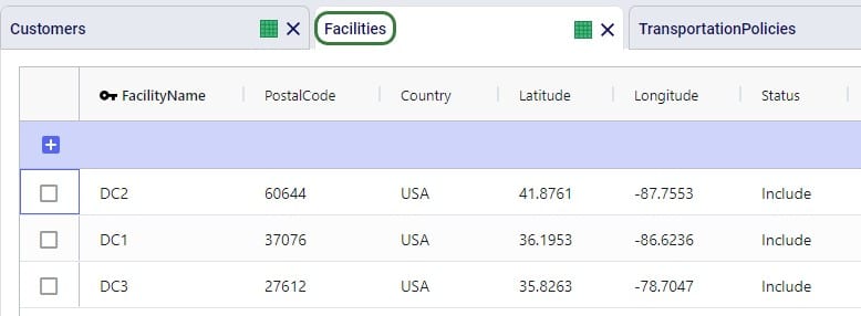
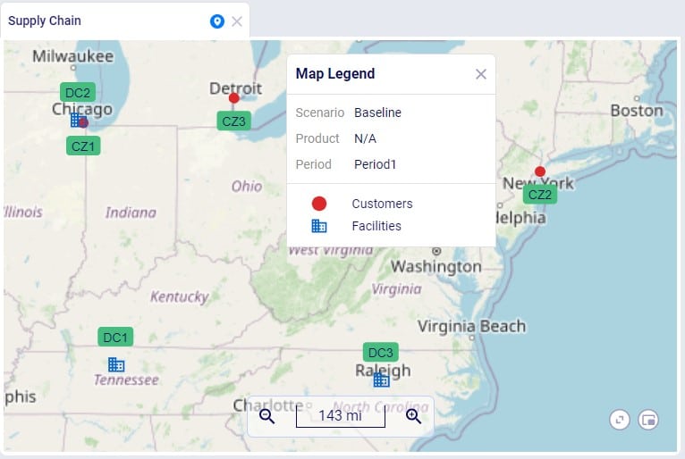
To facilitate model building, this model uses groups for Customer and DCs, as shown in the next screenshot. All DCs are members of the DCs group and all CZs are members of the Customers group:
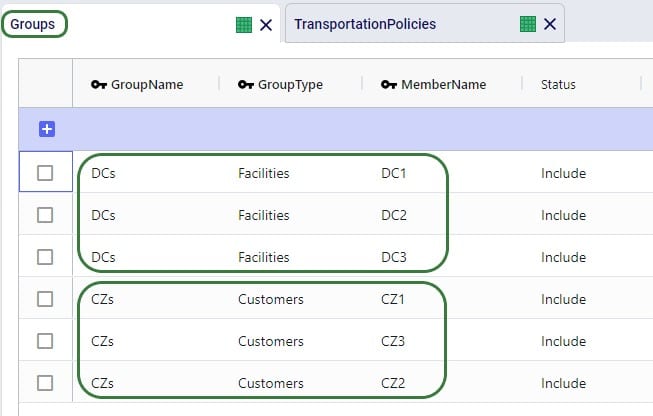
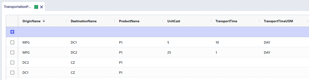
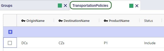
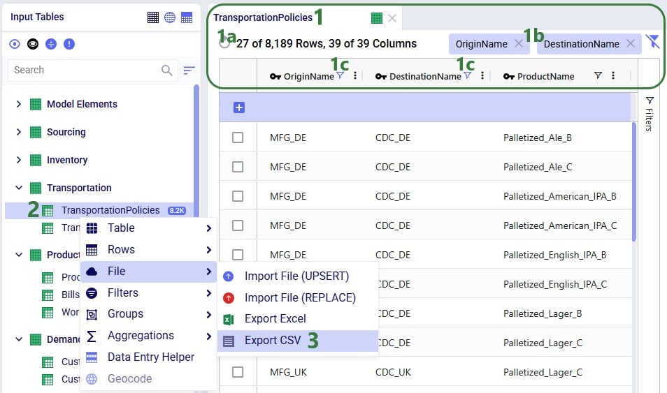
Using these groups, the Transportation Policies table is easily set up with 1 record from the DCs group to the CZs group as shown in the next screenshot. At runtime this 1 record is expanded into all possible OriginName-DestinationName combinations of the group members. So, this is an all DCs to all Customers policy that covers 9 possible origin-destination combinations.
Besides these tables, this simple model also has several other tables that are populated:
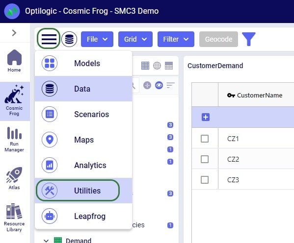
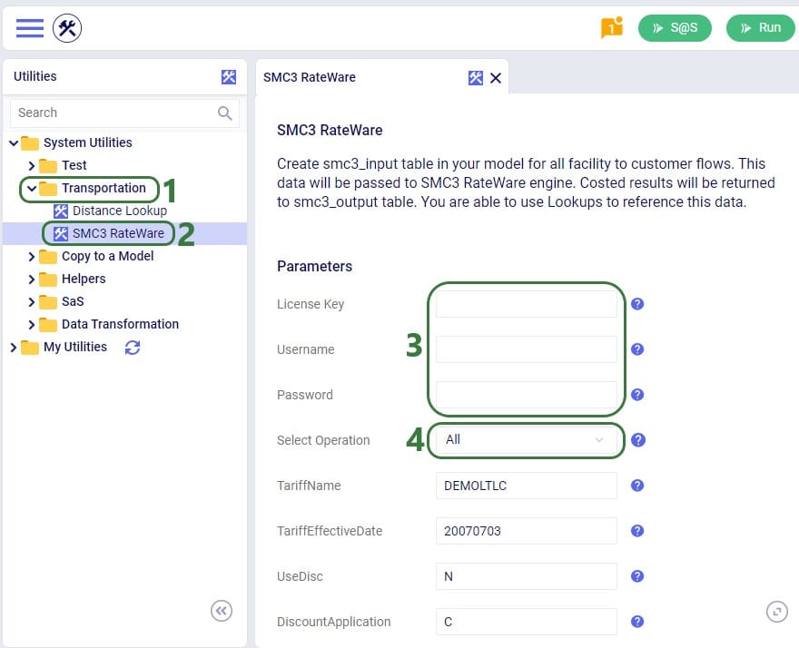
The SMC3 RateWare Utility is available by default from the Utilities module in Cosmic Frog, see next screenshot. Click on the Module Menu icon with 3 horizontal bars at the top left in Cosmic Frog, then click on Utilities in the menu that pops up:
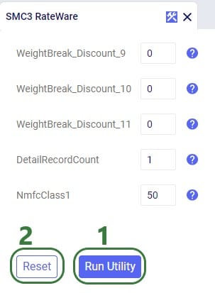
You will now see a list of Utilities, similar to the one shown in this next screenshot (your Utilities are likely all expanded, whereas most are collapsed in this screenshot):
The rest of the inputs that can be configured are specific to the RateWare XL LTL Rating Engine and we refer user to SMC3’s documentation for the configuration of these settings.
When the utility is finished running, we can have a look at the smc3_inputs and smc3_outputs tables (if the option of All was used for Select Operation). First, here is a screenshot of the smc3_inputs table:

The next screenshot shows the smc3_outputs table in Optilogic’s SQL Editor. This is also a table with many columns as it contains origin and destination information, repeats the inputs of the utility, and contains details of the retrieved rates. Here, we are only showing the 3 most relevant columns: originname (the source DC), destinationname (the customer), and detailrate_1 which is the retrieved LTL rate:

Now that we have used the SMC3 RateWare Utility to retrieve the LTL rates for our 9 origin-destination pairs, we need to configure the model to use them as they are currently only listed in the smc3_outputs custom table. We use the Lookups table (an Input table in the Functional Tables section) to create a lookup link between the smc3_outputs custom table and the Transportation Policies input table, as follows:
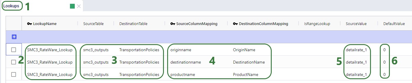
To finalize setting up the Lookup, we now apply it to the UnitCost field on the TransportationPolicies table, where we set the field to the name of the Lookup, see screenshot below. Now, when the model is run, the 1 transportation policy is expanded into the 9 origin-destination pairs it represents and the Unit Cost field is populated with the detailrate_1 value of the smc3_outputs table based on matching origin name, destination name, and product name between the 2 tables.

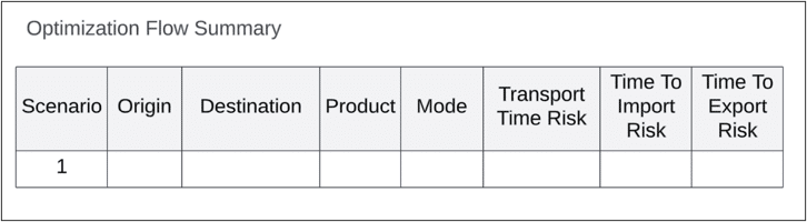
Lastly, we run a network optimization (NEO engine) on our small example model and look at the Optimization Flow Summary output table:
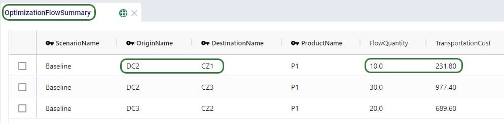
The optimization has correctly used DC2 as the source for CZ1 as it has the lowest rate for going to CZ1 of the 3 DCs (see screenshot further above of the smc3_outputs table). The rate is 23.18 and for 10 units moved (FlowQuantity) this results in a TransportationCost of 231.80. Similarly, we can double-check that indeed DC2 has the cheapest rate for going to CZ3 as well, DC3 has the cheapest rate for going to CZ2, and the Transportation Costs are correctly calculated as the LTL rate * flow quantity.
The Resource Library is the application within the Optilogic platform where you can find files that will help facilitate, accelerate, and customize your model building and running. These include Cosmic Frog template models, Python scripts, Reference Data and more.
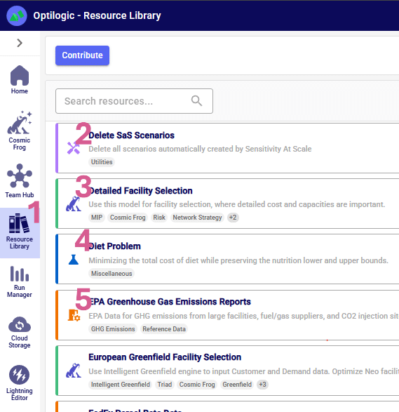
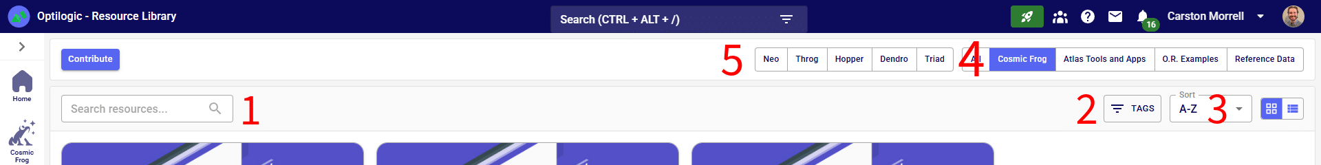
There are several ways to search, sort and filter the list of resources:
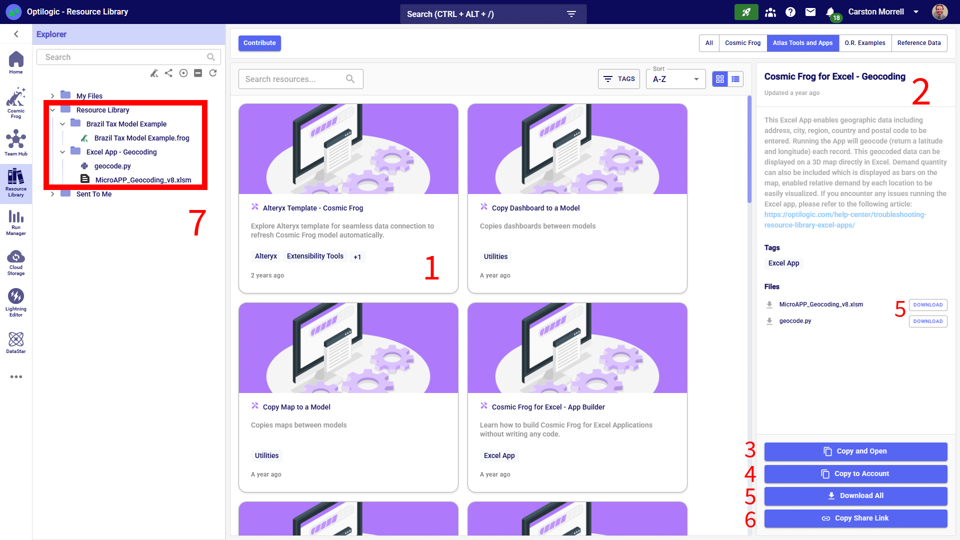
When a file in the list is selected by clicking on it, a Preview is shown on the right-hand side of the screen. This preview contains a short description of the resource, may contain a Video Introduction explaining for example the business problem or Cosmic Frog features covered in the resource, lists any Related (= included) Files, and lists any Tags that are associated with the resource so users can quickly understand what materials are covered by this resource.
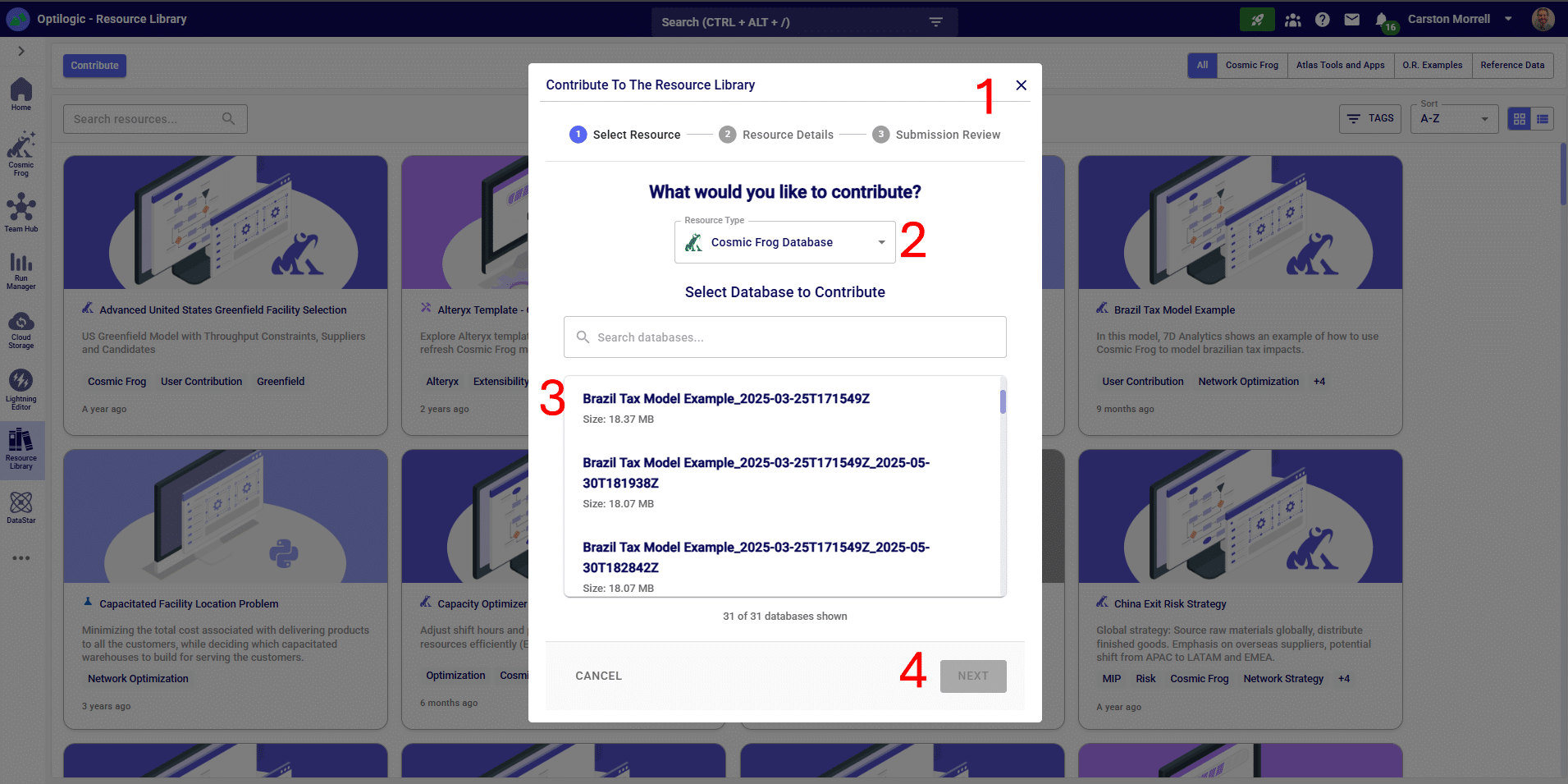
You may want to add a new resource to the Resource Library if you think other users may be interested in the contents, for example to showcase a certain business problem modelled in Cosmic Frog, or to add Reference Data that can be helpful for others too, or to share the automation of a common model building/analysis step. On other occasions you may want to replace a resource in the library with an updated version. If you want to add or replace a resource in the library, you can do so by clicking on the Contribute button (found in the top-left corner of the Resource Library), and then follow the steps as explained in the next sections.
After clicking the Contribute button the following submission form will be shown:
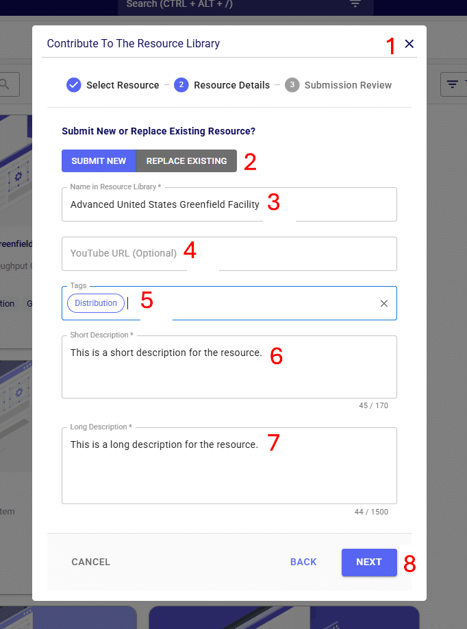
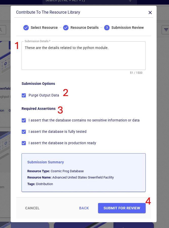
The steps to contribute a Python Module to the Resource Library are very similar to those described above for adding a Cosmic Frog database:
If you find that the standard constraints or costs in a model don’t quite capture your specific needs, you can create and define your own variables to use with costs and constraints.
To help in framing this discussion, let’s start with a simple example that fits into the standard input tables.
We wouldn’t need to do anything special in this instance, just create policies as normal and attach a Unit Cost of 5 to the MFG > DC transportation policy. To apply the constraint, we would create a Flow Constraint that sets a Max flow of 1000 units. While the input requirements are straightforward in this instance, let’s define both objectives in terms of variables as the solver would see them.
Flow Variable: MFG_CZ_Product_1_Flow
This example is simple, but it is important to think about costs and constraints in terms of the variables that they are applied over. This becomes even more important when we want to craft our own variables.
Let’s modify the constraint in the example above to now restrict the flow of Product_1 between MFG and DC to be no more than the flow of Product_2. Again, we will represent this in terms of variables as the solver will see them.
Flow Variables: MFG_CZ_Product_1_Flow, MFG_CZ_Product_2_Flow
We no longer have a constant on the right-hand side of our constraint – this is an issue as we have no way to input this type of a constraint requirement into the Flow Constraints table. Whenever we find ourselves expressing constraints or costs in terms of other variables that will be determined based on the model solve, we will need to make use of User Defined Variables.
Continuing with the constraint above, let’s modify the inequality statement so that we do in fact have a constant on the right-hand side. We can do this by subtracting one of the variables from both sides of the statement – this will then leave the right-hand side as 0.
We now have a constraint that can be modelled but we need to be able to define the left-hand side through the User Defined Variables table. User Defined Variables are defined as a series of Terms which are all linked to the same Variable Name. Each Term can be thought of as a solver variable as we have defined them in the examples above. For each Term, we will also need to enter a Coefficient, the Type of behavior we want to be capturing, and all of the needed information in the columns that follow depending on the Type that was just selected. All of these columns are based off of the individual constraint tables, so it is helpful to think about data as if you were entering a row in the specific constraint table.
Here is how the inputs for our example would look set up as a User Defined Variable:
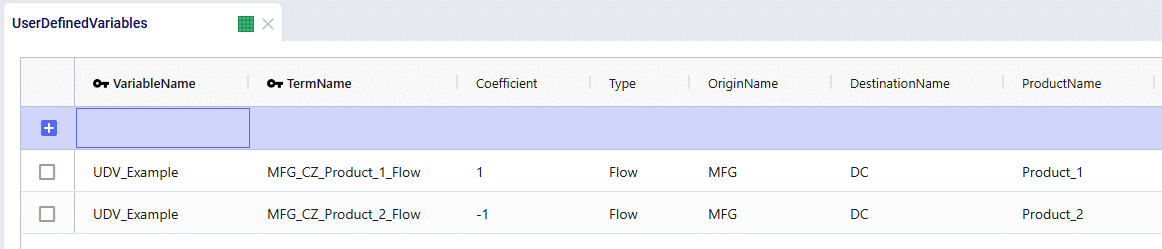
We can see that by using the coefficients of 1 and -1, we have now accurately built the left-hand side of our inequality statement. All that’s left is to link this to a User Defined Constraint.
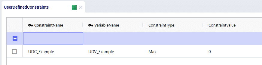
User Defined Constraints can be used to add restrictions to the values captured by the User Defined Variables. All that is needed is to enter the corresponding Variable Name and then select the appropriate constraint type and value.
Revisiting our inequality statement once more, we can see how the User Defined Constraint should be built:
MFG_CZ_Product_1_Flow – MFG_CZ_Product_2_Flow <= 0
Watch the video to learn how to import, export, geocode, and work with data within Cosmic Frog:
If you want to follow along, please download the data set available here:
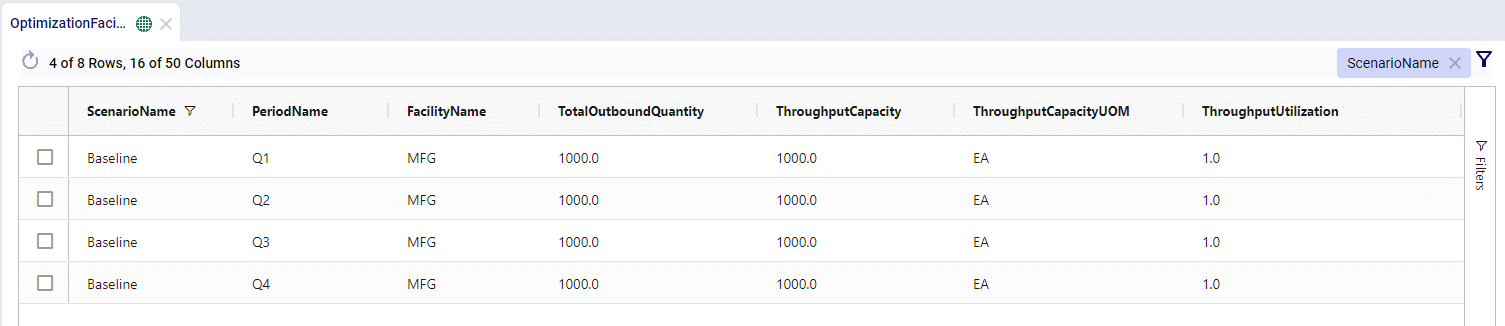
The Multi Time Period (MTP) tables allow for you to enter time-period specific data across many input tables. These MTP tables will act as overrides in the relevant periods for the records in their standard tables. If a record with the same key structure does not exist in the standard table, the MTP record won’t be recognized by the solver and will be dropped.
For example, we have a manufacturing facility with a throughput capacity of 1000 units. When this information is entered into the Facilities table, the throughput capacity will be used for each period in the model:
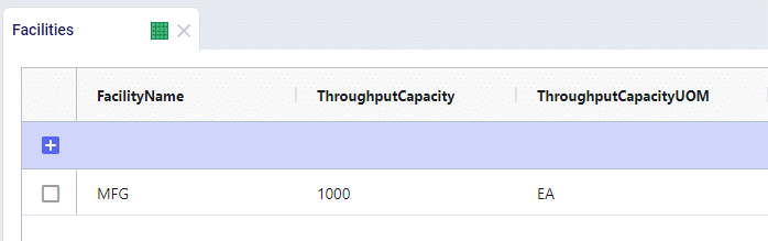
Let’s say that the manufacturing facility is expanding operations over the year and wants to show that the throughput capacity gradually increases over each quarter. This adjustment in throughput capacity can be defined in the Facilities Multi Time Period table:

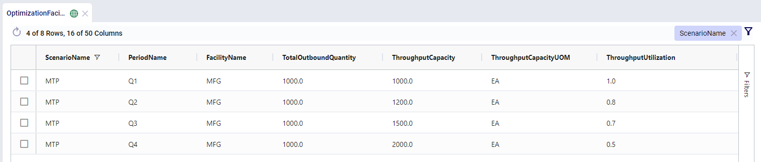
We can see that the throughput capacity increased over time and given the constant outbound quantity, the throughput utilization goes down as the model progresses.
In all of the policy multi-time period tables, there are two fields which appear to be similar – Status and Policy Status.
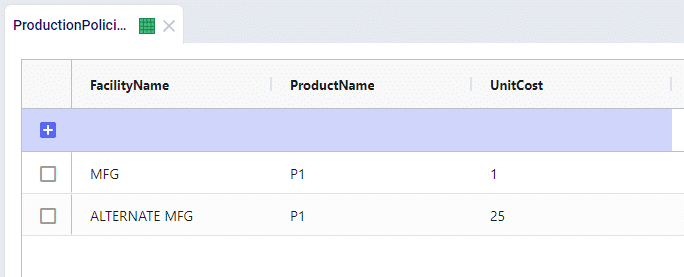
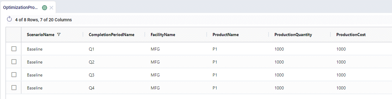
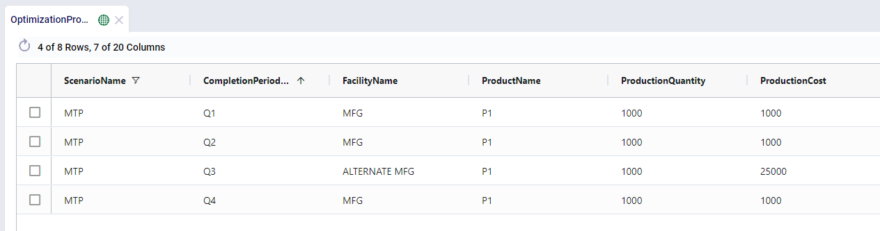
For example, we have 2 manufacturing locations that can produce the same product at very different costs. We’ll see that the MFG location is used as the sole production option as it is far cheaper.
Now let’s say that we have to shut production down at the MFG location for maintenance in Q3, we can do this through the Production Policies Multi Time Period table:
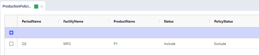
This can be a quick way to to adjust policies over different times and is an alternative to using constraints. The use of Policy Status in place of constraints will stop the creation of extra solver variables as well as reducing the number of constraints being placed over the solution. This can help contribute to better model performance.
Similar to how Status and Policy Status work, you have the ability to change the operating status of a Facility and a Work Center over time. This would allow you to Open, Close, or Consider the use of a Facility or Work Center in any given period.
Using the same example as above, we can model the maintenance at MFG during Q3 by closing the entire location:
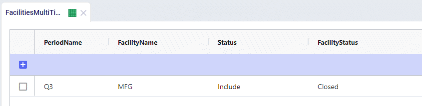
Closing the entire facility will do more than just limit production, the facility is then completely removed from the network for that given period and no other activities can take place.
Watch the video to learn how to connect your data tool of choice directly to your Optilogic model:
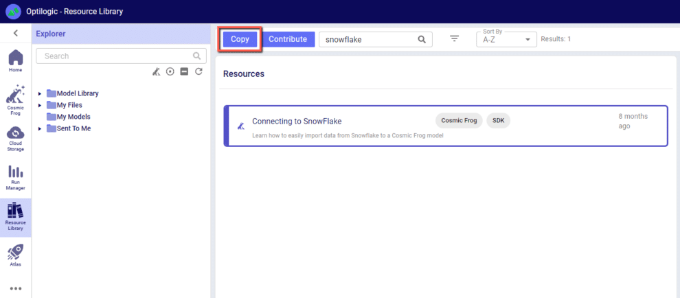
An example of how to connect a Cosmic Frog model to a Snowflake database, along with a video walkthrough, can be found in the Resource Library. To get a copy of this demo into your own Optilogic account simply navigate to the Resource Library and copy the Snowflake template into your workspace.
The following instructions show how to establish a local connection, using Alteryx, to an Optilogic model that resides within our platform. These instructions will show you how to:
Watch the video for an overview of the connection process:
A step by step set of instructions can also be downloaded in the slide deck here: CosmicFrog-Alteryx-Connection-Instructions
To make a local connection you must first open a Firewall connection between your current IP address and the Optilogic platform. Navigate to the Cloud Storage app – note that the app selection found on the left-hand side of the screen might need to be expanded. Check to see if your current IP address is authorized and if not, add a rule to authorize this IP address. You can optionally set an expiration date for this authorization.
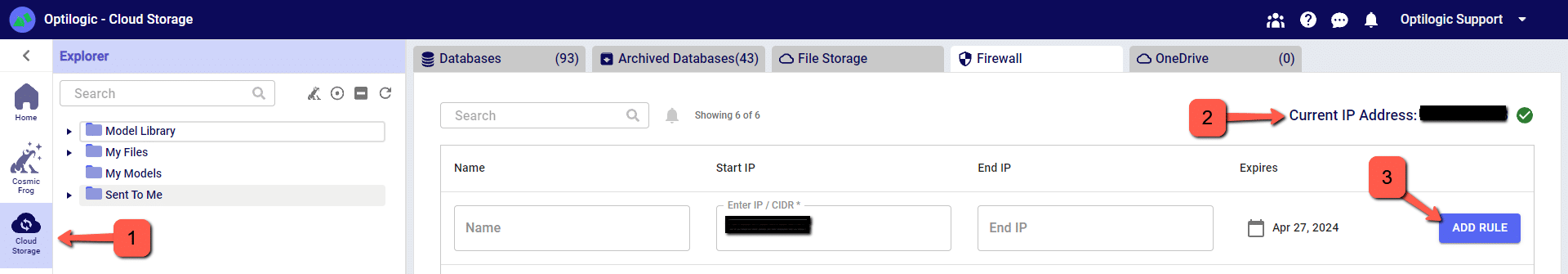
If you are working from a new IP Address, a banner notification should be displayed to let you know that the new IP Address will need to be authorized.
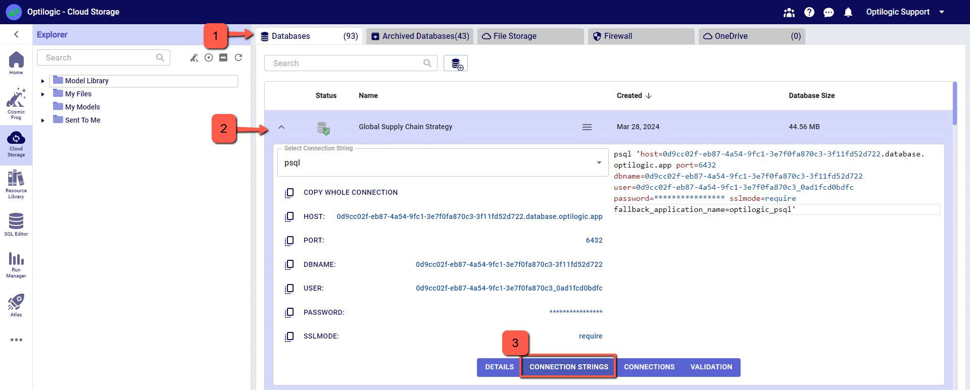
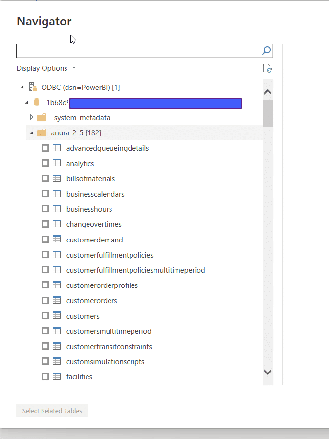
From the Databases section of the Cloud Storage page, click on the database that you want to connect to. Then, click on the Connection Strings button to display all of the required connection information.
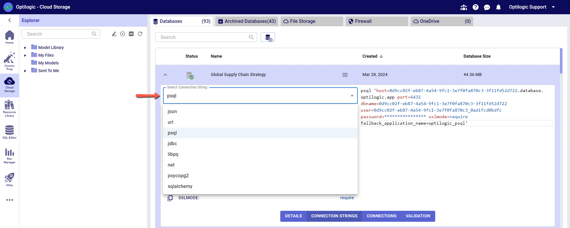
We have connection information for the following formats:
To select the format of your connection information, use the drop-down menu labeled Select Connection String:
For this example, we will copy and paste the strings for the ‘PSQL’ connection. The screen should look something like the following:
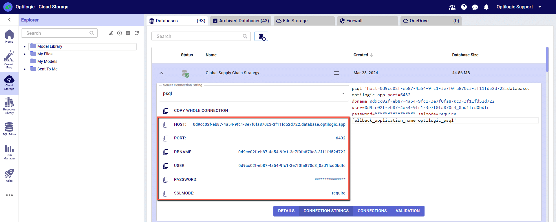
You can click on any of the parameters to copy them to your clipboard, and then paste them into the relevant field when establishing the PSQL ODBC connection.
Many tools, including Alteryx, use Open Database Connectivity (ODBC) to enable a connection to the Cosmic Frog model database. To access the Cosmic Frog model, you will need to download and install the relevant ODBC drivers. Latest versions of the drivers are located here: https://www.postgresql.org/ftp/odbc/releases/
From here, click on the latest parent folder, which as of June 20, 2024 will be REL-16_00_0005. Select and download the psqlodbc_x64.msi file.
When installing, use the default settings from the installation wizard.
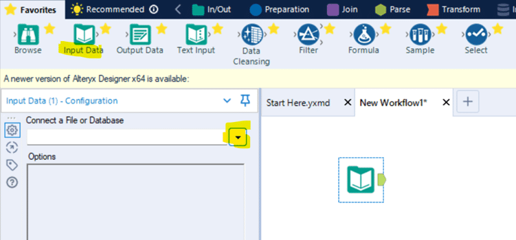
At this point we have the pieces to make a connection in Alteryx. Open Alteryx and start a new Workflow. Drag the Input Data action into the Workflow and click to “Connect a File or Database.”
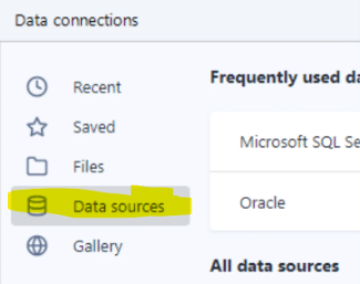
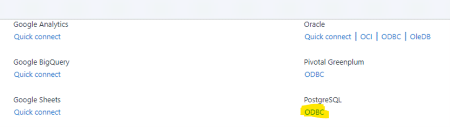
Select “Data sources” and scroll down to select “PostgresSQL ODBC”
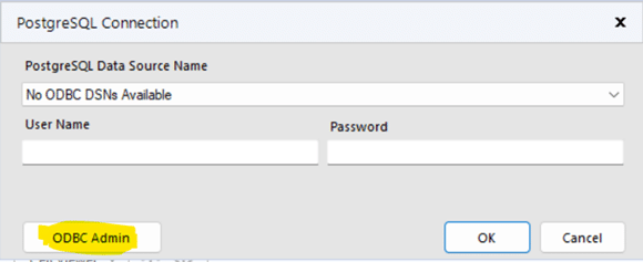
On the next screen click “ODBC Admin” to setup the connection.
Click “Add” to create a new connection and then select “PostgreSQL ANSI(x64)” then click “Finish.”

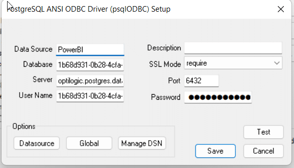
Now we need to configure the connection with the information we gathered from the connection strings.
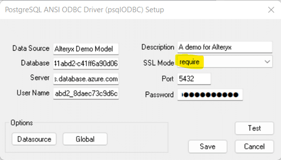
“Data Source” and “Description” allow you to name the connection, these can be named whatever you wish.
Copy the values for “Server”, “Database”, “User Name”, “Password” and “Port” from the connection string information copied from Optilogic Cloud Storage (see above).
DON’T FORGET to select “require” in “SSL Mode”
You may click “Test” to confirm the connection works or click “Save.”
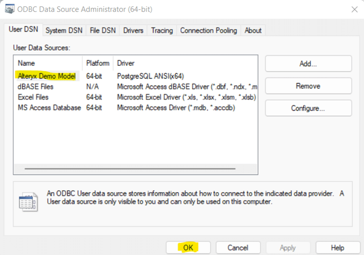
Now select the new connection, in this example “Alteryx Demo Model” and click “OK”
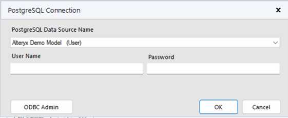
Now we need to select the same Data Source that we just built in ODBC within Alteryx. We need to enter the username and password for the connection for Alteryx authentication. These are the same credentials used to setup the ODBC connection. Remember to use your specific model’s credentials from the Connection String in the Optilogic platform Cloud Storage page.
Depending on your organization’s security protocols, one additional step might need to be taken to whitelist Optilogic’s Postgres SQL Server. This can be done by whitelisting the host URL (*.postgres.database.azure.com) and the port (6432). If you are unsure how to whitelist the server or do not have the necessary permissions, please contact your IT department or network administrator for assistance.
11/16/2023 – There is an issue connecting through ODBC with the latest version of Alteryx. While we await a fix in an updated version of Alteryx, you can still connect with an older version of Alteryx (2021.4.2.47884)
05/01/2024 – Alteryx has resolved the ODBC connection issue with their latest major version release of 2024.1. If your currently installed Alteryx version is not working as intended, please upgrade to latest.
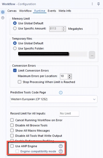
An alternative workaround is to disable the AMP engine on your Alteryx workflow. For any workflows that use the ODBC connection to a database hosted on the platform, you can uncheck the option in the Workflow Configuration for ‘Use AMP Engine’. The Workflow Configuration window will display on the left side of your screen if you click on the whitespace anywhere in your workflow.
The following instructions show how to establish a local connection, using Azure Data Studio, to an Optiogic model that resides in the platform. These instructions will show you how to:
Watch the video for an overview of the connection process:
To make a local connection you must first open a Firewall connection between your current IP address and the Optilogic platform. Navigate to the Cloud Storage app – note that the app selection found on the left-hand side of the screen might need to be expanded. Check to see if your current IP address is authorized and if not, add a rule to authorize this IP address. You can optionally set an expiration date for this authorization.
If you are working from a new IP Address, a banner notification should be displayed to let you know that the new IP Address will need to be authorized.
From the Databases section of the Cloud Storage page, click on the database that you want to connect to. Then, click on the Connection Strings button to display all of the required connection information.
We have connection information for the following formats:
To select the format of your connection information, use the drop-down menu labeled Select Connection String:
For this example, we will copy and paste the strings for the ‘PSQL’ connection. The screen should look something like the following:
You can click on any of the parameters to copy them to your clipboard, and then paste them into the relevant field in Azure Data Studio when establishing the PSQL connection.
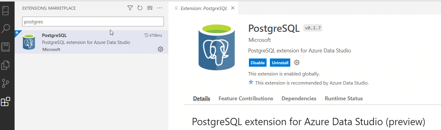
Within Azure Data Studio click the “Extensions” button and type in “postgres” in the search box to find and install the PostgreSQL extension.
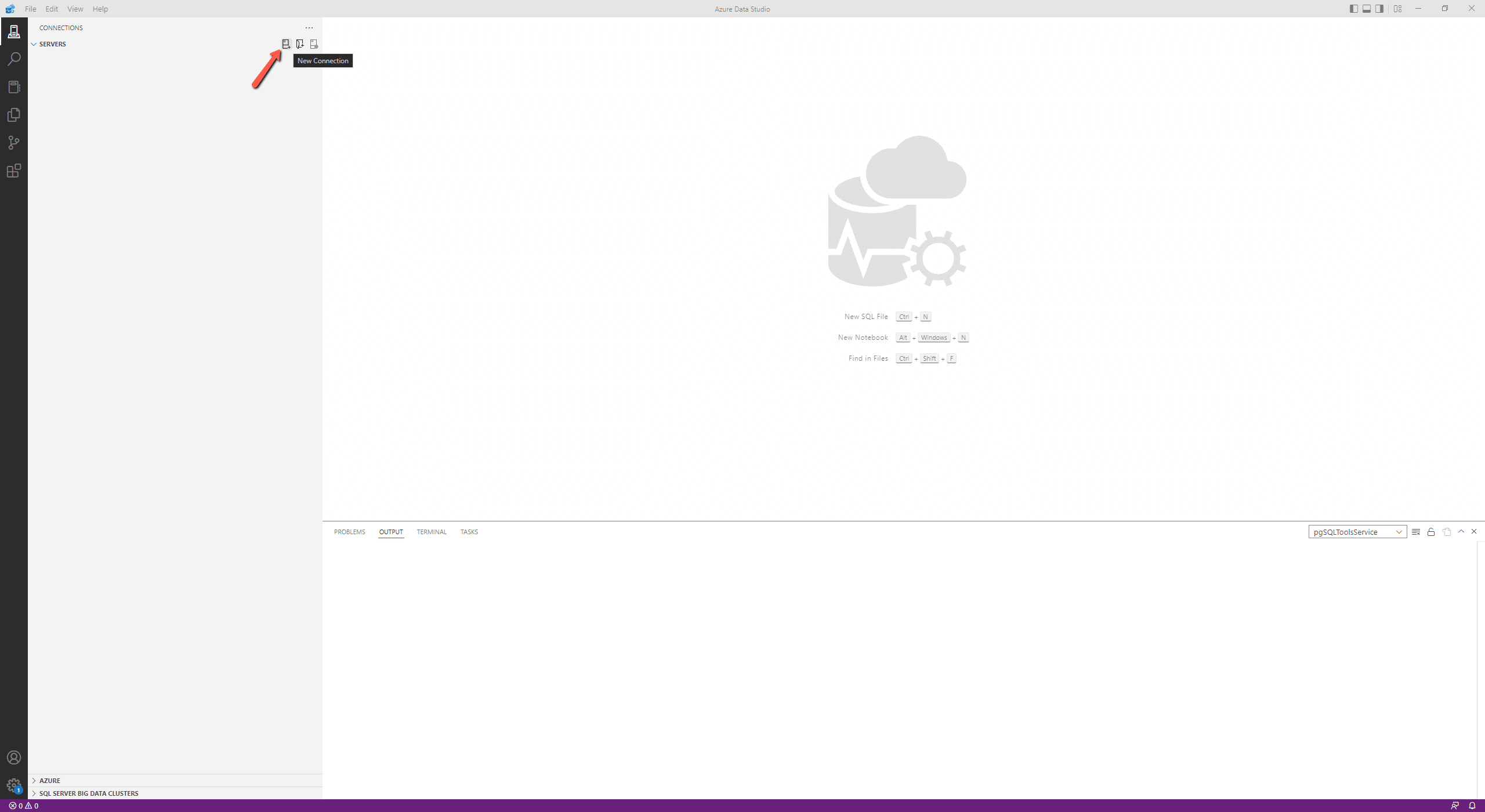
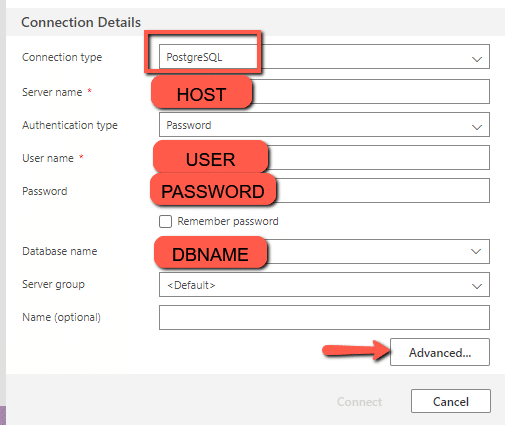
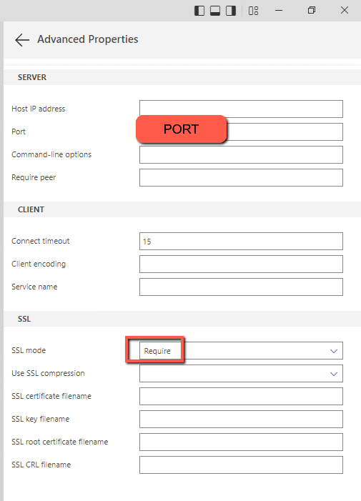
Add a new connection in Azure Data Studio, change the connection type to “PostgreSQL, “and enter the arguments for “PSQL” from the Cloud Storage page. NOTE: you will need to click “Advanced” to type in the Port and to change the SSL mode to “require.”
Depending on your organization’s security protocols, one additional step might need to be taken to whitelist Optilogic’s Postgres SQL Server. This can be done by whitelisting the host URL (*.database.optilogic.app) and the port (6432). If you are unsure how to whitelist the server or do not have the necessary permissions, please contact your IT department or network administrator for assistance.
The following instructions show how to establish a local connection, using Power BI, to an Optilogic model that resides within our platform. These instructions will show you how to:
To make a local connection you must first open a Firewall connection between your current IP address and the Optilogic platform. Navigate to the Cloud Storage app – note that the app selection found on the left-hand side of the screen might need to be expanded. Check to see if your current IP address is authorized and if not, add a rule to authorize this IP address. You can optionally set an expiration date for this authorization.
If you are working from a new IP Address, a banner notification should be displayed to let you know that the new IP Address will need to be authorized.
From the Databases section of the Cloud Storage page, click on the database that you want to connect to. Then, click on the Connection Strings button to display all of the required connection information.
We have connection information for the following formats:
To select the format of your connection information, use the drop-down menu labeled Select Connection String:
For this example, we will copy and paste the strings for the ‘PSQL’ connection. The screen should look something like the following:

You can click on any of the parameters to copy them to your clipboard, and then paste them into the relevant field when establishing the PSQL ODBC connection.
Many tools, including Alteryx, use Open Database Connectivity (ODBC) to enable a connection to the Cosmic Frog model database. To access the Cosmic Frog model, you will need to download and install the relevant ODBC drivers. Latest versions of the drivers are located here: https://www.postgresql.org/ftp/odbc/releases/
From here, click on the latest parent folder, which as of June 20, 2024 will be REL-16_00_0005. Select and download the psqlodbc_x64.msi file.
When installing, use the default settings from the installation wizard.
Within Windows, open the ODBC Data Sources App (hint search: “ODBC” in your Windows spotlight search).
Click “Add” to create a new connection and then select “PostgreSQL ANSI(x64)” then click “Finish.”
Enter the details from your Cloud Storage connection — (hint: click to copy/paste)
You may click “Test” to confirm the connection works or click “Save.”
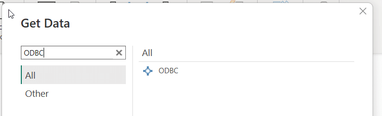
Open Power BI and select “Get data from another source”

Enter “ODBC” in the Get Data window and select connect
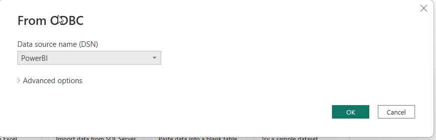
Select your Database connection from the dropdown and click OK
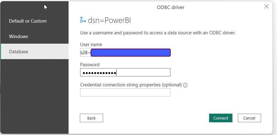
Enter your username and password one last time from the Cloud Storage page
Select the tables you wish to see and use within PowerBI
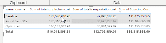
Create Dashboards of Data from Cosmic Frog tables!
If you are comfortable with traditional linear programming techniques, you can select the “Write Input Solver Files” and “Write LP File” parameters to get useful output files.

After running, these files are in your file explorer.
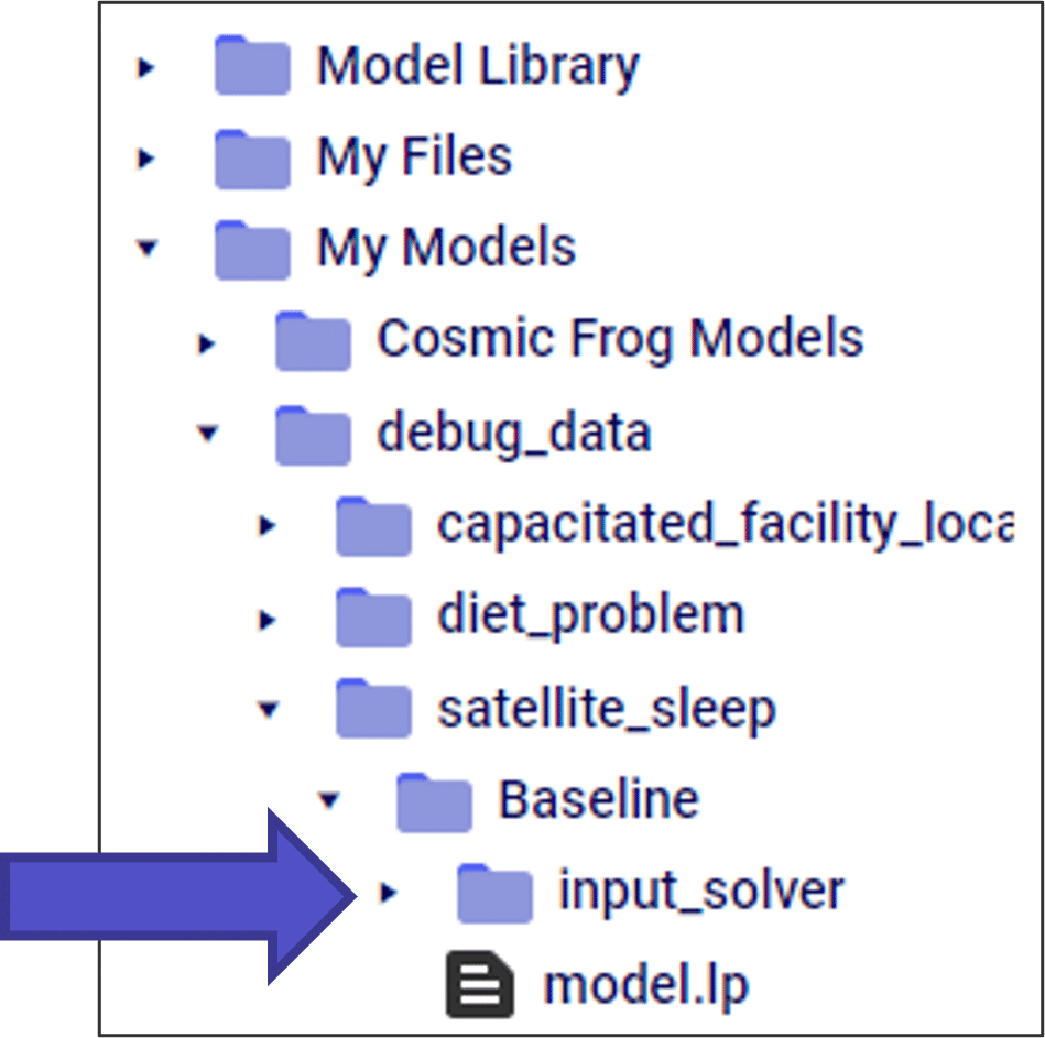
The “input_solver” folder has a list of all the tables that are entered into the optimization solver. This is useful for:
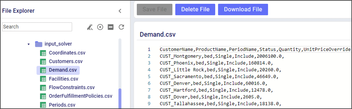
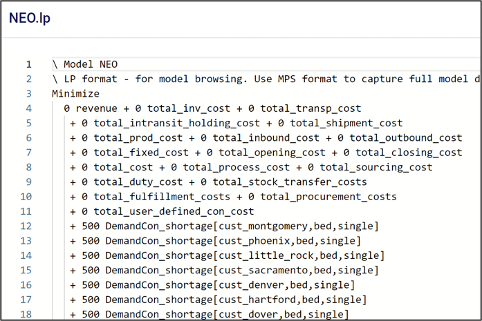
The “model.lp” file shows the model in a more traditional MIP optimization format, including the objective function and model constraints.

When using the Infeasibility Diagnostic engine, the LP file is different than a traditional Neo run. In this case, the cost coefficients in the objective function are set to 0. Instead, a positive cost coefficient is added to each slack constraint, and the goal of the model is to minimize the slack values. This allows us to find the “edge” of infeasibility.
After every Cosmic Frog run, it’s a great habit to check the OptimizationValidationErrorReport table. Even for models that run successfully, this table can have useful information on how the input data is being processed by the solver.
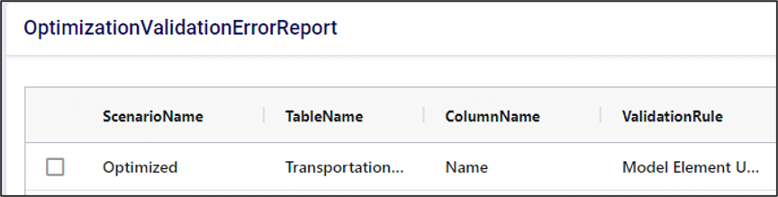
Key columns in the validation error report can tell you:
Validation errors that have “high” or “moderate” severity are likely to cause an infeasible model. In fact, Cosmic Frog has an “infeasibility checker” that looks for these kinds of errors and flags them before running the model to save you run time.
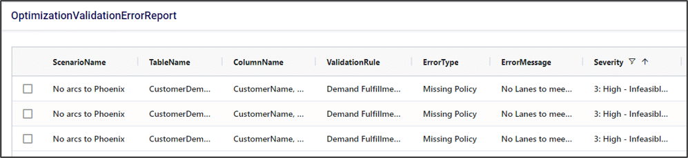
In this example, there are no transportation lanes that can deliver beds to CUST_Phoenix, so demand cannot be fulfilled. The infeasibility checker finds this and stops the model run before it even tries to optimize.
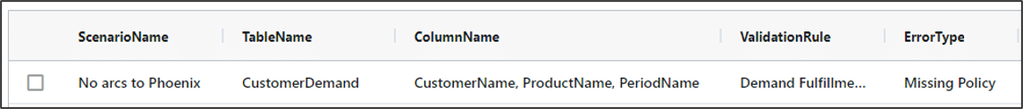

A couple of examples of how we could fix this error:
The OutputValidationErrorReport table is often very useful, even if a model “successfully” runs. This table will catch potential errors that do not cause infeasibility but could change the model results. In this example, there is a typo in the CustomerDemand table for “CUST_Montgomery”. Here, the model drops that row in the demand table. This will not cause an infeasible model, as it just removes that demand constraint. However, it means that no product will be sent to this customer in our optimized result.
Cosmic Frog supports importing and exporting both CSV and Excel files directly through the application. This enables users to for example:
In this documentation we will cover how users can import and export data into and out of Cosmic Frog, and illustrate this with multiple examples.
There are 2 methods of importing Excel/CSV data into Cosmic Frog’s input tables available to users:
Pointers on how data to be imported needs to be formatted will be covered first, including some tips and call outs of specifics to keep in mind when using the upsert import method. Next, the steps to import a CSV/Excel file will be walked through step by step.
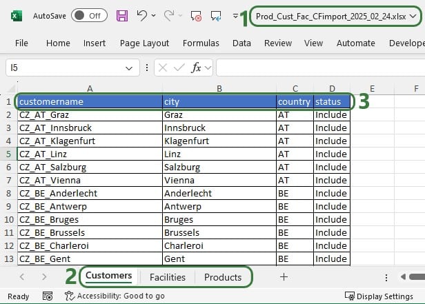
Data is mapped from CSV/Excel files based on matching column names and table names matching to the file name (CSV) or worksheet name (Excel):
Data preparation tips:
CSV vs Excel: CSV files only have 1 “worksheet”, so it can only contain data to be imported into 1 table, whereas Excel files can have multiple worksheets with data to be imported to different tables in Cosmic Frog.
Please take note of how existing records are treated when using the upsert import method to import to a table which already has some data in it:
We will illustrate these behaviors through several examples too.
Users can import 1 or multiple CSV or Excel files simultaneously, please take note of how the import will work for following situations:
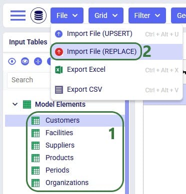
Once ready to import the prepared CSV/Excel file(s), user has 2 ways of accessing the import and export methods: from the File menu in the toolbar and from the right-click context menu of an input table. It looks like this from the File menu to import a file:
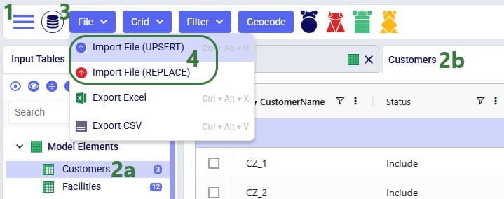
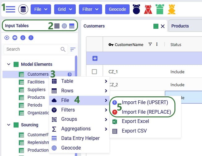
And when using the right-click context menu the steps to import a file are as follows:
When using the replace import method, a confirmation message will now be shown on which user can click Import to continue the import or Cancel to abort.
Next, a file explorer window opens in which user can browse to and select the CSV/Excel file(s) to import:
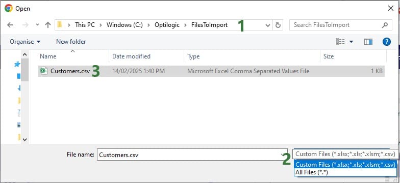
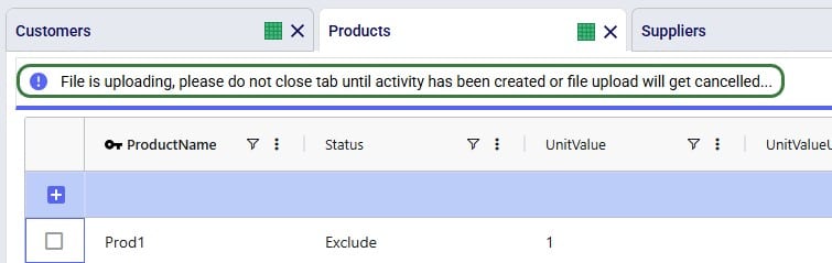
Once the import starts, a status message shows at the top of the active table:
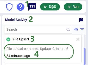
The Model Activity log will also have an entry for each import action:
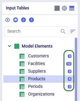
User can see the results of the import by opening and inspecting the affected input table(s), and by looking at the row counts for the tables in the input tables list, outlined in green in this screenshot:
A common way to start building a new model in Cosmic Frog is to make use of the replace import method to populate multiple tables simultaneously with data from Excel or CSV files. These files have typically been prepared from ERP extracts which have been manipulated to match the Cosmic Frog table and column names. This way, users do not need to enter data manually into the Cosmic Frog input tables, which would be very laborious. Note that it can be helpful to first export empty tables from a new, empty Cosmic Frog model to have a template to start filling out (see the “Exporting to CSV/Excel Files” section further below on how to do this).
Starting with an empty new model in Cosmic Frog:
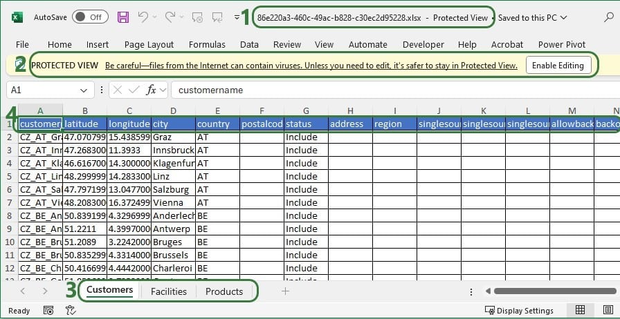
User has prepared the following Excel .xlsx file:
After importing this file into Cosmic Frog, we notice that the Customers, Facilities and Products tables now have row counts that match the number of records we had in the Excel file that was used for the import, and we can open the individual tables to see the imported records:

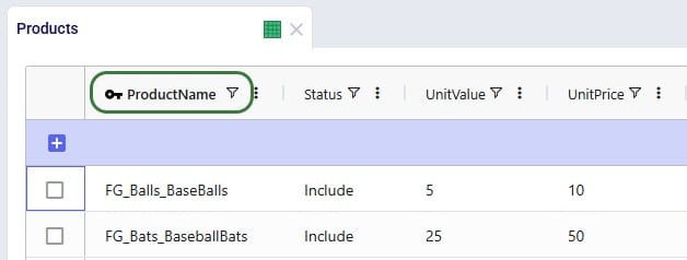
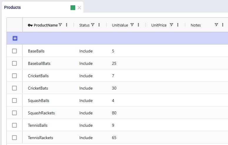
Consider user is modelling a sports equipment company and has populated the Products table of a Cosmic Frog model with 8 products as follows:
After working with the model for a while, the user realizes a few things:
As item number 1 will change the product names, a column that is part of the primary key of the Products table, user will need to use the replace import method to make these changes as the upsert method does not change the values of columns that are part of the primary key. Following is the .xlsx file user prepares to replace the data in the Products table with:

After importing the file using the replace method, the Products table looks like this:
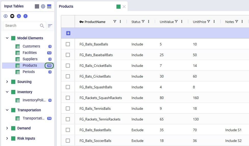
We see the records are the exact same as what was contained in the Products.xlsx file that was imported, and the row count for the Products table has correctly gone up to 10 with the 2 new products added.
Continuing from the Products table in the last screenshot above, user now wants to make a few additional changes as follows:
To make these changes to the Products table, the user prepares the following Products file to be upserted to the Products table, where the green numbers in the screenshot below match the items described in the bullet point list directly above:

After using the upsert import method for this file into the Products table, it contains following records. The ones changed / added are listed at the bottom:

In the boxes outlined in green we see that all the expected changes and the insertion of the 1 new record have been made.
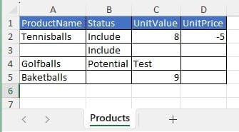
Let us also illustrate what will happen when files with invalid /missing data are imported. We will use the replace import method for the example here, but similar results will be seen when using the upsert method. Following screenshot shows a Products table that has been prepared in Excel, where we can see several issues already: a blank Product Name, a negative value for Unit Price, etc.
After this file is imported to the Products table using the replace method, the Products table will look as follows:
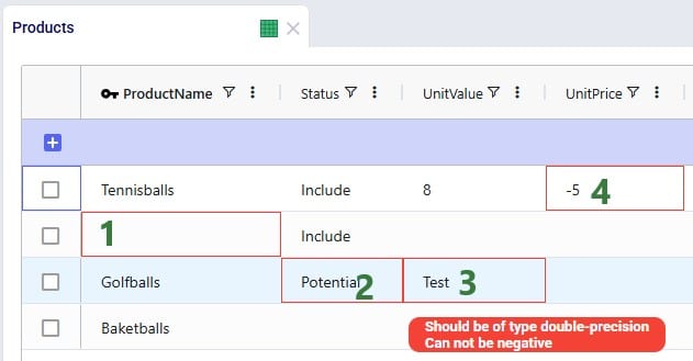
The cells that are outlined in red contain invalid values. Hovering over each cell will show a tooltip message describing the problem.
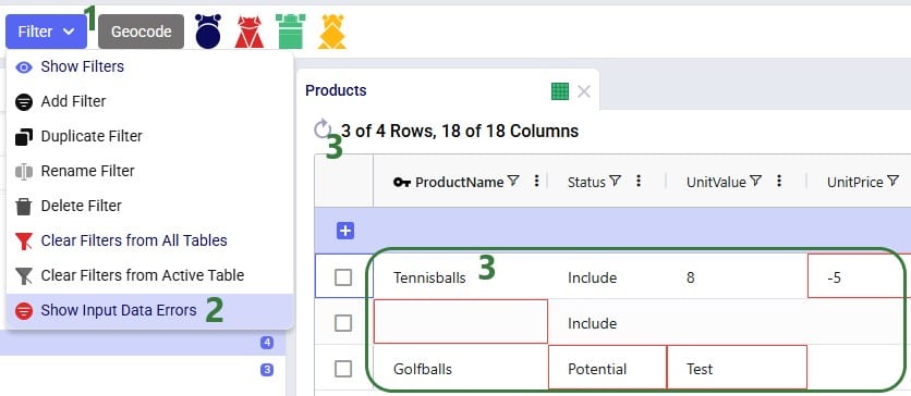
For tables with many records, it may be hard to find the fields in red outline manually. To help with this, there is a standard filter user can apply that will show all records that have 1 or multiple input data errors:
In conclusion, Cosmic Frog will let a user import invalid data, and then helps user identify the data issues with the red outlines, hover over tooltips, and the Show Input Data Errors filter.
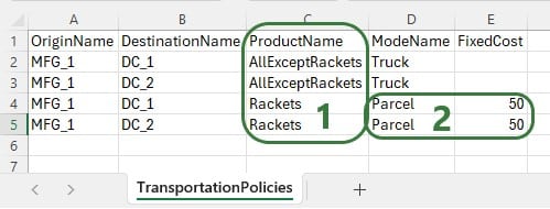
Consider following Transportation Policies table:
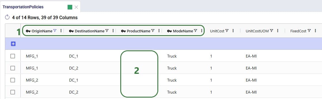
There is now a change where from MFG_1 all Racket products need to be shipped by Parcel for a fixed cost of $50. User creates 2 Named Filters (see the Named Filters in Cosmic Frog help center article) in the Products table: 1 that filters out all racket products (those products that have a product name that start with FG_Racket) which is named Rackets and 1 that filters out all non-racket products (those products that do not contain racket in the product name) which is named AllExceptRackets. Next, user prepares following TransportationPolicies.csv file to upsert into the Transportation policies table with the intention to update the first 2 records in the existing table to be specific for the AllExceptRackets products and add 2 new ones for the Rackets products:
The result of using this file to upsert to the Transportation Policies table is as follows:
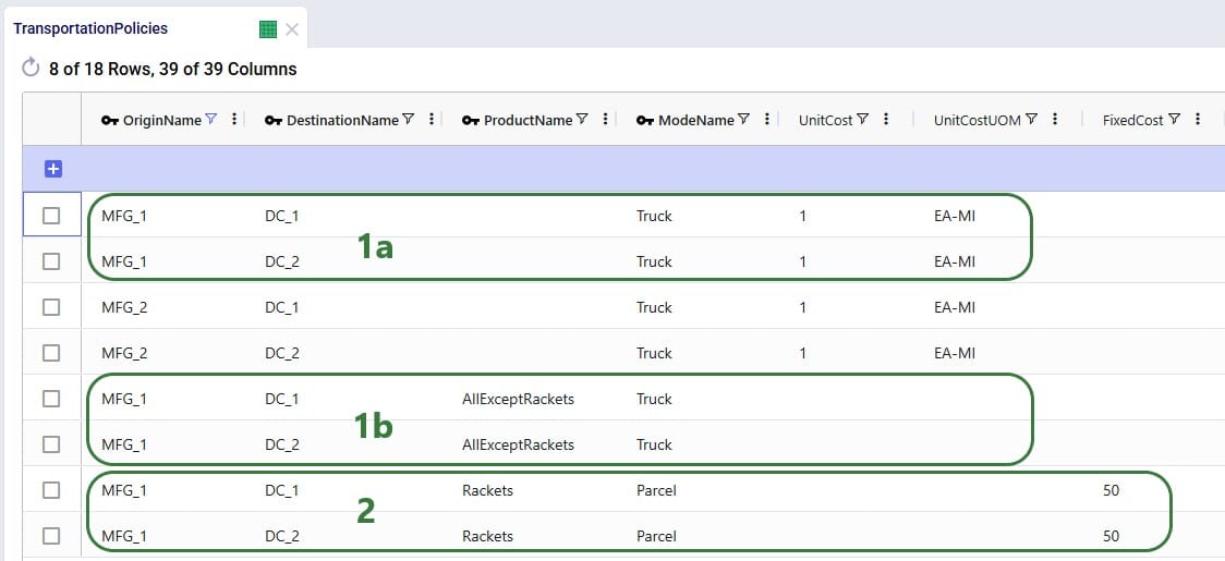
This example shows that users need to be mindful of which fields are part of the table’s primary key and remember that values of primary key fields cannot be changed by the upsert import method. An example workflow that will achieve the desired changes to the Transportation Policies table is as follows:
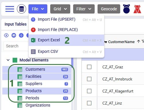
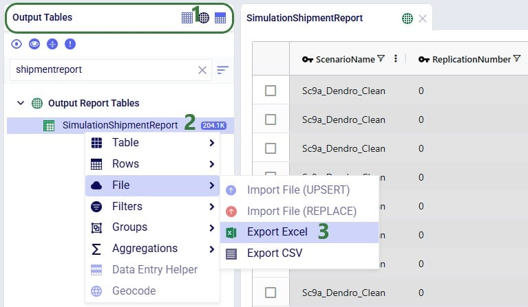
It is possible to export a single table or multiple tables (input and output tables) to CSV or Excel from Cosmic Frog. Similar to importing data from CSV/Excel, user can access the export options in 2 ways: from the File menu in the toolbar and from the context menus that come up when right-clicking on tables in the input/output/custom tables lists.
Please note:
The steps to export multiple tables to an Excel file are as follows:
Once the export starts, following message appears at the top of the active table:

Once the export is complete, the exported file can be found in the folder where user’s downloaded files are saved:
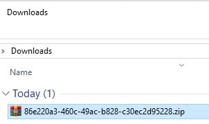
When exporting multiple tables to Excel or CSV, the downloaded file will be a .zip file with an automatically generated name based on the model’s Cosmic Frog ID. Extracting the zip-file will show an .xlsx file of the same name, which can be opened in Excel:
These are the steps to export multiple tables to CSV:

When the export starts, the same “File is exporting…” message as shown in the previous section will be showing at the top of the active table. Once the export process is finished, the exported file can again be found in the folder where user’s downloaded files are saved:
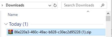
The file is again a zip-file, and it has the same name based on the model’s Cosmic Frog ID, just appended with (1), as there is already a zip-file of the same name in the Downloads folder from the previous export to Excel. Unzipping the file creates a new sub-folder of the same name in the Downloads folder:

Exporting a single table to Excel can also be done from the File menu, in the same way as multiple tables are exported to Excel, which was shown above in the “Export Multiple Tables to Excel” section. Now, we will show the second way of doing this by using the context menu that comes up when right-clicking on a table:
When the export starts, the same “File is exporting…” message as shown above will be showing at the top of the active table. Once the export process is finished, the exported file can again be found in the folder where user’s downloaded files are saved:

The name of the exported CSV file matches that of the table that was exported.
Exporting a single table to CSV can also be done from the File menu, in the same way as multiple tables are exported to CSV, which was shown above in the “Export Multiple Tables to CSV” section. Now, we will show the second way of doing this by using the context menu that comes up when right-clicking on a table:
When the export starts, the same “File is exporting…” message as shown above will be showing at the top of the active table. Once the export process is finished, the exported file can again be found in the folder where user’s downloaded files are saved:
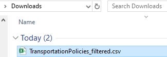
For single tables exported to CSV, the name of the file is the same as the name of the exported table. If the Cosmic Frog table was filtered, the file name is appended with “_filtered” like it is here to remind user that only the filtered rows are contained in this exported file.
This video guides you though creating your free account and the features of the Optilogic Cosmic Frog supply chain design platform.
If you are running into issues receiving your account confirmation email, please see the troubleshooting article linked here.
Greenfield analysis (GF) is a method for determining the optimal location of facilities in a supply chain network. The Greenfield engine in Cosmic Frog is called Triad and this name comes from the oldest known species of frogs – Triadobatrachus. You can think of it as the starting point for the evolution of all frogs, and it serves as a great starting point for modeling projects too! We can use Triad to identify 3 key parameters:
GF is a great starting point for network design—it solves quickly and can reduce the number of candidate site locations in complicated design problems. However, a standard GF requires some assumptions to solve (e.g. single time period, single product). As a result, the output of a Triad model is best suited as initial information for building a more robust Cosmic Frog optimization (Neo) or simulation (Throg) model.
You can run GF in any Cosmic Frog model. Running a GF model only requires two input tables to be populated:

A third important table for running GF is the Greenfield Settings table in the Functional Tables section of the input tables. We call our GF approach “Intelligent Greenfield” because of the different parameters available by configuring this settings table. The Greenfield Settings table is always populated with defaults and users can change these as needed. See the Greenfield Setting Explained help article for an explanation of the fields in this table.
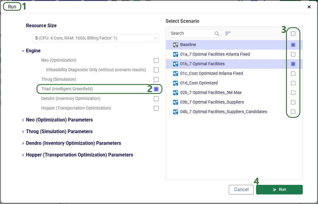
A greenfield analysis starts with clicking the “Run” button at the right top of the Cosmic Frog application, just like a Neo or Throg model.

After clicking on the Run button, the Run screen comes up:
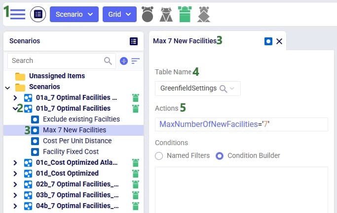
Besides making changes to values in the Customers and/or Customer Demand tables, GF scenarios often make changes to 1 or multiple settings on the Greenfield Settings table. The next screenshot shows an example of this:
To improve the solve speed of a Triad model, we can use customer clustering. Customer clustering reduces the size of the supply chain by grouping customers within a given geometric range into a single customer. We can set the clustering radius (in miles) in the Greenfield Settings table in the Customer Cluster Radius column.

Clustering is optional, and leaving this column blank is the same as turning off clustering.
While grouping customers can significantly improve the run time of the model, clustering may result in a loss of optimality. However, Greenfield is typically used as a starting point for a future Neo optimization model, so small losses in optimality at this phase are typically manageable.
The only constant is change. When building our supply chains, the “optimal” design doesn’t only mean lowest cost. What happens if (or perhaps when) a disruption occurs? Fragile, low-cost supply chains can end up costing more in the long run if they aren’t resilient to the dynamic nature of today’s world.
We believe that optimality includes resilience. That’s why every Cosmic Frog run includes a risk rating from our DART risk engine.
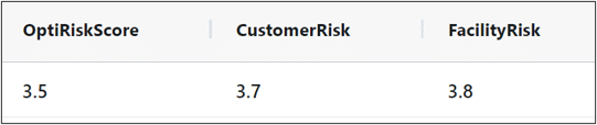
Every Cosmic Frog run outputs an Opti Risk score. The Opti Risk score is an aggregate measure of the overall supply chain risk. It includes the following sub-categories:
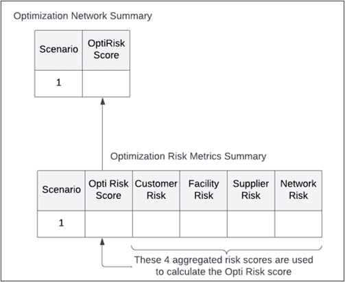
After running a model, you can find the Opti Risk score (as well as the scores for each of the sub-categories) in the output risk tables. The Opti Risk score can also be found in the OptimizationNetworkSummary table.
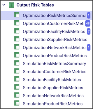
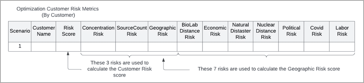
The overall Customer Risk score is an aggregation of each individual customer’s risk described in the OptimizationCustomerRiskMetrics or SimulationCustomerRiskMetrics tables. In each scenario, there is one risk score per customer per period.
Each customer risk score includes:
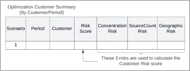
For each sub-category, the geographic risk score is also an aggregation of several risk factors:
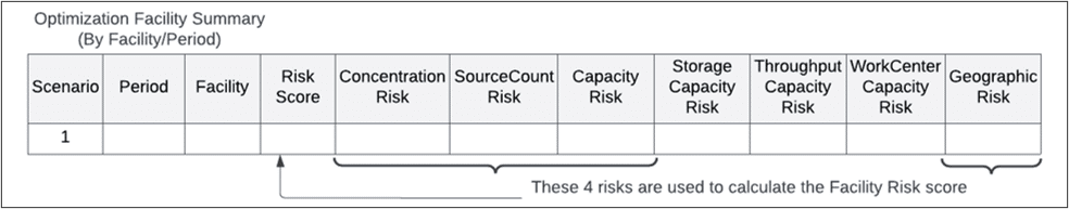
Like the customer risk score, the overall facility risk score is an aggregation of risk across all facilities in your supply chain. In the FacilityRiskMetric tables, there is an individual risk score per facility per period.
The facility risk score includes:
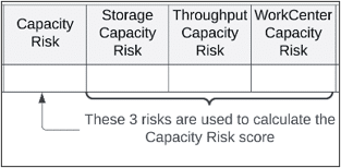
The capacity risk has three sub-components:
The facility geographic risk has the same components as the customer geographic risk.
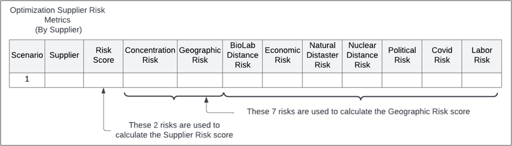
The supplier risk is calculated per supplier per period and includes:
Both the concentration and geographic risks include the same elements as described previously.
Network risk differs from the other risk scores in that it is not tied to a specific supply chain element. There is only one network risk score per scenario, and it includes:
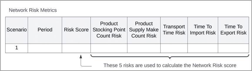
The transport and import/export time risks are aggregated across individual origin/destination pairs for every product and transport mode. The individual risk scores can be found in the OptimizationFlowSummary table.
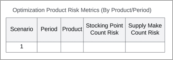
The stocking point count and supply make count risks are aggregations across every product and period. The individual risk scores can be found in the ProductRiskMetrics tables.
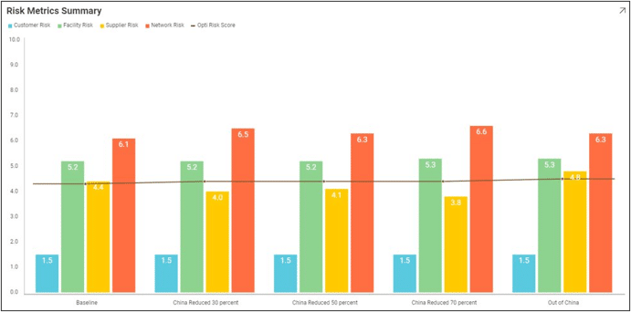
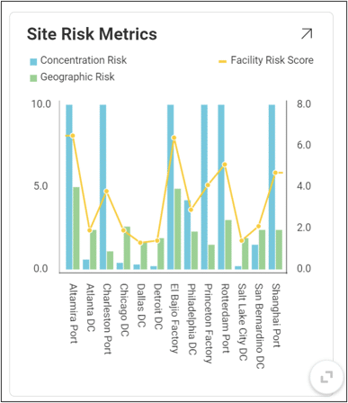
We can use our visualization tools to get a better sense of how risk varies across design scenarios.
With Optilogic’s new Teams feature set (see the "Getting Started with Optilogic Teams" help center article) working collaboratively on Cosmic Frog models has never been easier: all members of a team have access to all contents added to that team’s workspace. Centralizing data using Teams ensures there is a single source of truth for files/models which prevents version conflicts. It also enables real-time collaboration where files/models are seamlessly shared across all team members, and updates to any files/models are instantaneous for all team members.
However, whether your organization uses Teams or not, there can be a need to share Cosmic Frog models, for example to:
In this documentation we will cover how to share models, and the different options for sharing. Sharing models can be from an individual user or a team to an individual user or a team. As the risk of something undesirable happening with the model when multiple people work on it increases, it is important to be able to go back to a previous version of the model. Therefore, it is best practice to make a backup of a model prior to sharing it. Continue making backups when important/major changes are going to be made or when wanting to try out something new. How to make a backup of a model will be explained in this documentation too and will be covered first.
A backup of a model is a snapshot of its exact state at a certain point in time. Once a backup has been made, users can use them to revert to if needed. Initiating the creation of a backup of a Cosmic Frog model can be done from 3 locations within the Optilogic platform: 1) from the Models module within Cosmic Frog, 2) through the Explorer and 3) from within the Cloud Storage application on the Optilogic platform. The option from within Cosmic Frog will be covered first:
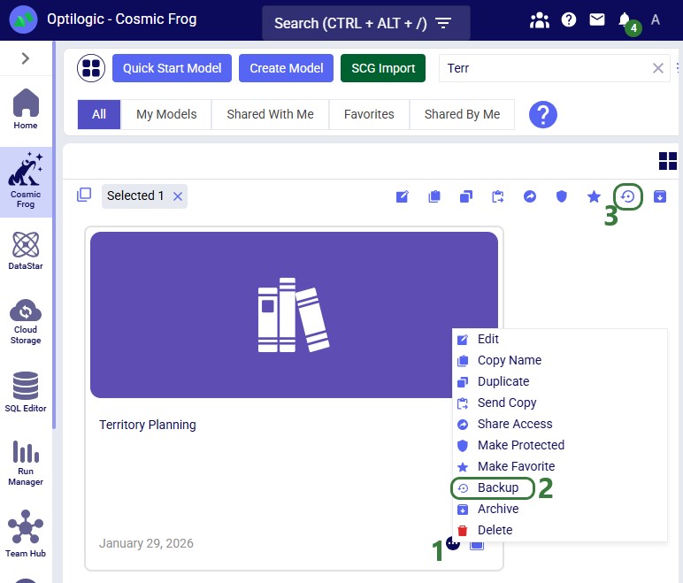
When in the Models module of Cosmic Frog (aka the Model Manager), hover over the model you want to create a backup for, and click on the icon with 3 horizontal dots that comes up at the bottom right of the model card (1). This brings up the model management options context menu, from which you can choose the Backup option (2). If only 1 model is selected, the Backup option can also be accessed from the toolbar at the top of the model list/grid (3).
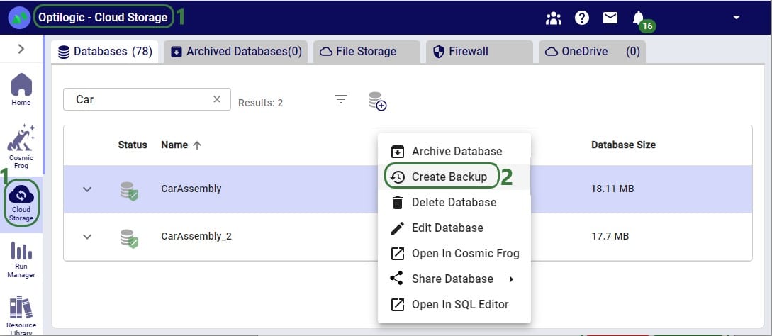
From the Cloud Storage application it works as follows:
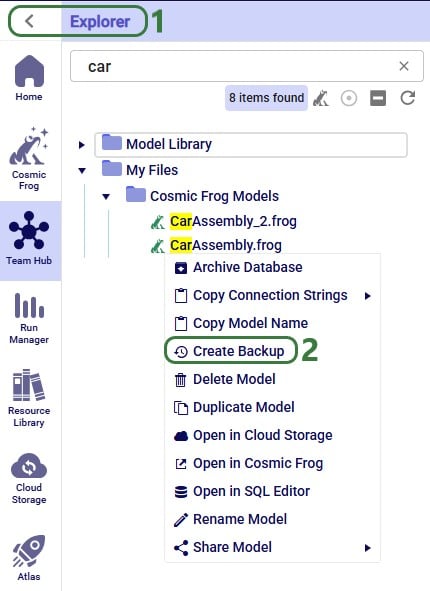
Through the Explorer, the process is similar:
Whether from the Models module within Cosmic Frog, through the Cloud Storage application or via the Explorer, in all 3 cases the Create Backup form comes up:
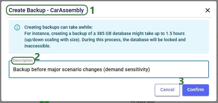
After clicking on Confirm, a notification at the top of the user’s screen will pop up saying that the creation of a backup has been started:

At the same time, a locked database icon with hover over text of “Backup in progress…” appears in the Status field of the model database (this is in the Cloud Storage application’s list of databases):

This locked database icon will disappear again once the backup is complete.
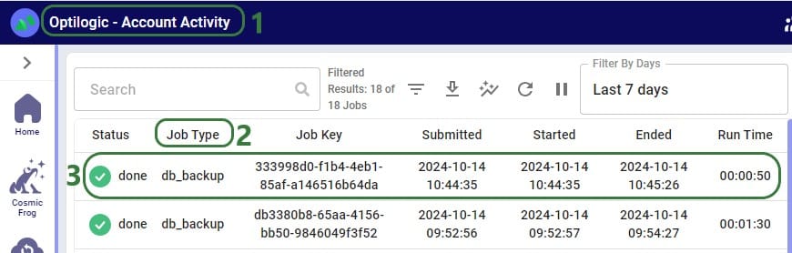
Users can check progress of the backup by going to the user’s Account menu under their username at the right top of the screen and selecting “Account Activity” from the drop-down menu:
To access any backups, users can expand individual model databases in the Cloud Storage application:

There are 2 more columns in the list of databases that are not shown in the screenshot above:

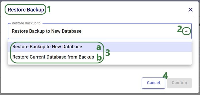
When choosing to restore a backup, the following form comes up:
Now that we have discussed how models can be backed up, we will cover how models can be shared. Note that it is best practice to make a backup of your model before sharing it.
If your organization uses Teams, first make sure you are in the correct workspace, either a Team’s or your personal My Account area, from which you want to share a model. You can switch between workspaces using the Team Hub application, which is explained in this "Optilogic Teams - User Guide" help center article.
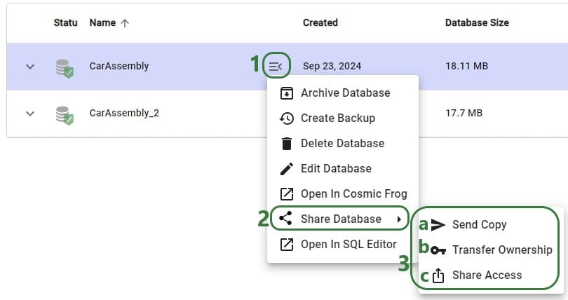
Like making a backup of a model database, sharing a model can also be done through the Cloud Storage application and the Explorer. Starting with the Cloud Storage option:
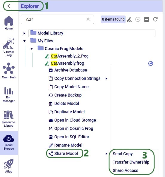
The Share Model options can also be accessed through the Explorer:
Now we will cover the steps of sending a copy of a model to another user or team. The original and the copy are not connected to each other after the model was shared in this way: updates to one are not reflected in the other and vice versa.

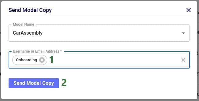
After clicking on the Send Model Copy button, a message that says “Model Copy Sent Successfully” will be displayed in the Send Model Copy form. Users can go ahead and send copies of other models to other user(s)/teams(s) or close out of the form by clicking on the cross icon at the right top of the form.
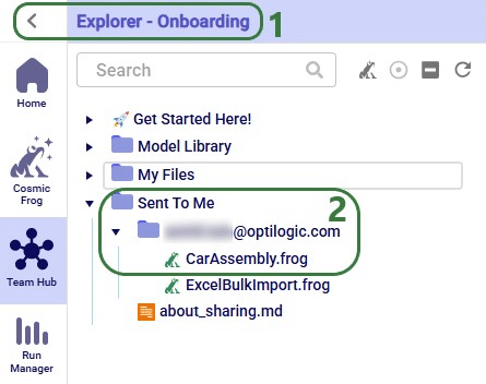
In this example, a copy of the CarAssembly model was sent to the Onboarding team. In the Onboarding team’s workspace this model will then appear in the Explorer:
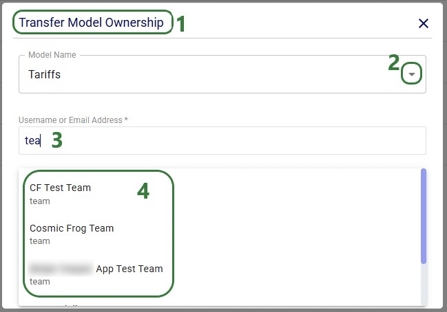
Next, we will step through transferring ownership of a model to another user or team. The original owner will no longer have access to the model after transferring ownership. In the example here, the Onboarding team will transfer ownership of the Tariffs model to an individual user.
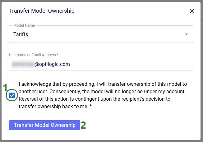
After clicking on the Transfer Model Ownership button, a message that says “Transferred Ownership Successfully” will be displayed in the Transfer Model Ownership form. Users can go ahead and transfer ownership of other models to other user(s)/teams(s) or close out of the form by clicking on the cross icon at the right top of the form.
There will be a notification of the model ownership transfer in the workspace of the user/team that performed the transfer:
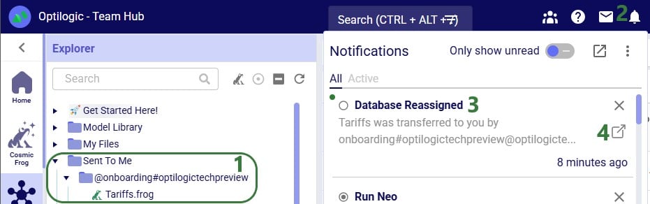
The model now becomes visible in the My Account workspace of the individual user the ownership of the model was transferred to:
Lastly, we will show the steps of sharing access to a model with a user or team. Note that Sharing Access to a model can be done from Explorer and from the Cloud Storage application (same as for the Send Copy and Transfer Ownership options), but can also be done from the Models module in Cosmic Frog:

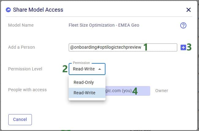
In Cosmic Frog's Models module (aka Model Manager), hover over the model card of the model you wan to share access to and then click on the icon with 3 horizontal dots that comes up in the bottom right of the model card (1). Clicking on this icon brings up the model management actions context menu, from which you can choose the Share Access option (2). If only 1 model is selected, the Share Access option is also available from the model management actions toolbar at the top of the model list/grid (3).
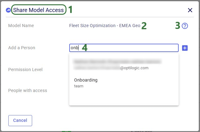
In our walk-through example, an individual user will share access to a model called "Fleet Size Optimization - EMEA Geo" with the Onboarding team.
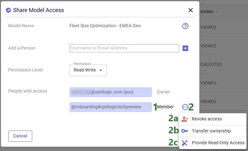
After the plus button was clicked to share access of the Fleet Size Optimization - EMEA Geo model with the Onboarding team, this team is now listed in the People with access list:
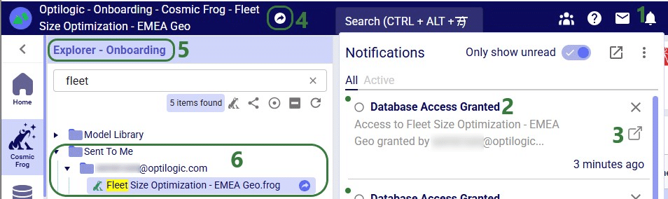
Now, in the Onboarding team’s workspace, we can access this model, of which the team receives a notification too:
Now that the Onboarding team has access to this model, they can share it with other users/teams too: they can either send a copy of it or share access, but they cannot transfer ownership as they are not the model’s owner.
In the Explorer of the workspace of the user/team who shared access to the model, a similar round icon with arrow inside it will be shown next to the model’s name. The icon colors are just inverted (blue arrow in white circle) and here the hover text is “You have shared this database”, see the screenshot below. There will also be a notification about having granted access to this model and to whom (not shown in the screenshot):

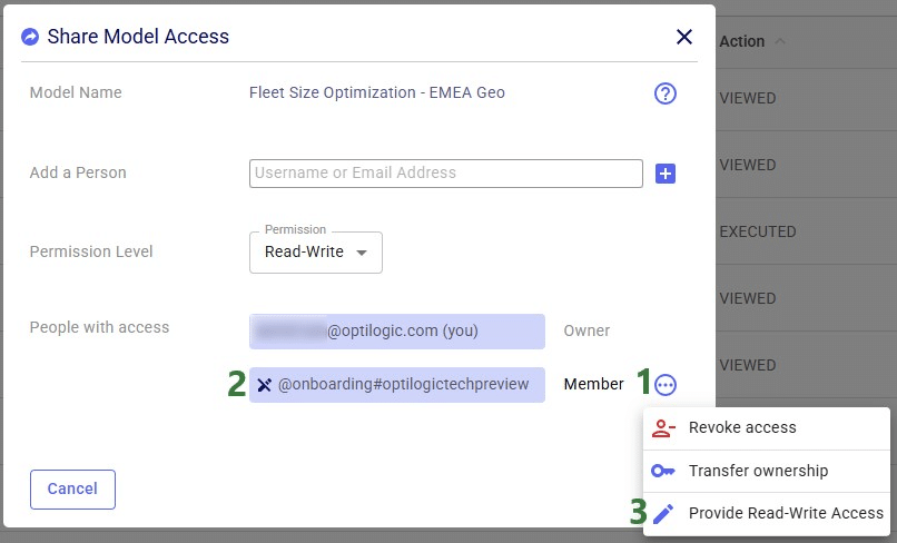
If the model owner decides to revoke access or change the permission level to a shared model, they need to open the Share Model Access form again by choosing Share Access from the Share Model options / clicking on the Share icon when hovering over the model's card on the Cosmic Frog start page:
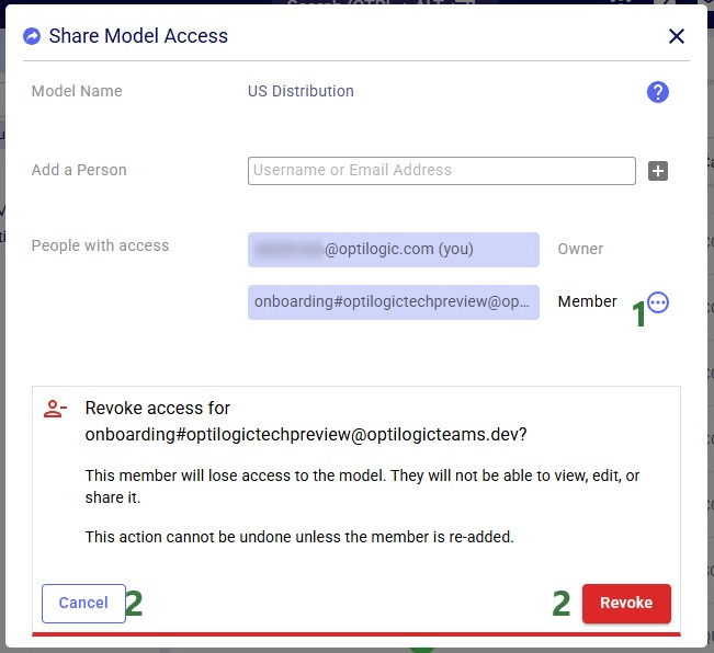
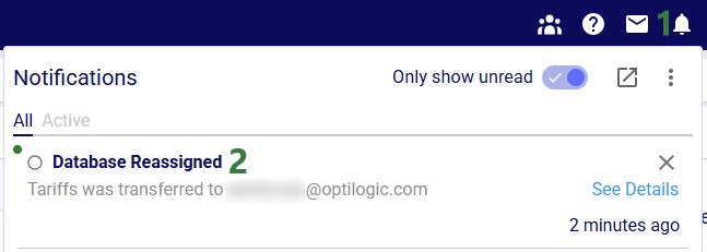
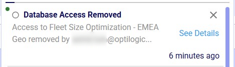
If access to a model is revoked, the team/user that was previously granted access but now no longer will have access, receives a notification about this:
With Read-Only access, teammates and stakeholders can explore a shared model, view maps, dashboards, and analytics, and provide feedback — all while ensuring that the data remains unchanged and secure.
Read-Only mode is best suited for situations where protecting data integrity is a priority, for example:
See the Appendix for a complete list of actions and whether they are allowed in Read-Only Access mode or not.
Similar to revoking access to a previously shared model, in order to change the permission level of a shared model, user opens the Share Model Access form again by choosing Share Access from the Share Model options / clicking on the Share icon when hovering over the model's card on the Cosmic Frog start page:
Models with Read-Only access can be recognized on the Optilogic platform as follows:
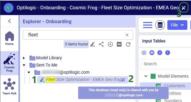
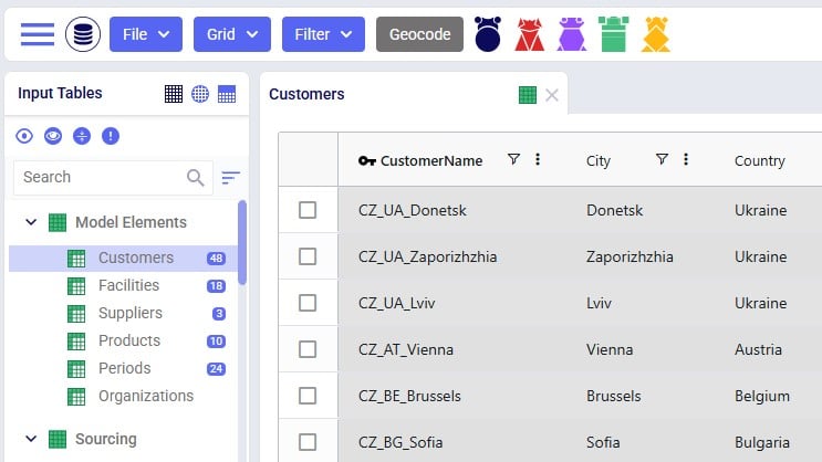
Input tables of Read-Only Cosmic Frog models are greyed out (like output tables already are by default), and and write actions (insert, delete, modify) are disabled:
Read-Only models can be recognized as follows in other Optilogic applications:
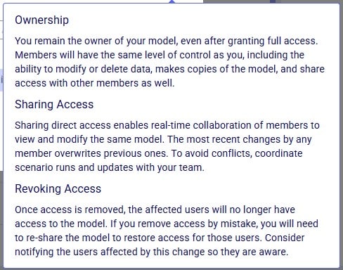
When working with models that have shared access, please keep following in mind:
In addition to the various ways model files can be shared between users, there is a way to share a copy of all contents of a folder with another user/team too:
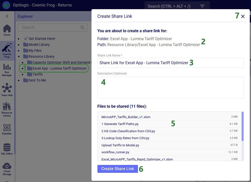
After clicking on the Create Share Link button, the share link is copied to the clipboard. A toast notification of this is temporarily displayed at the right top in the Optilogic platform. The user can paste the link and send it to the user(s) they want to share the contents of the folder with.
When a user who has received the share link copies it into their browser while logged into the Optilogic platform, the following form will be opened:
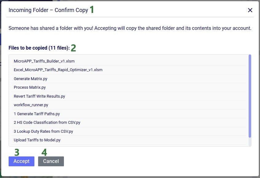
Folders copied using the share link option will be copied into a subfolder of the Sent To Me folder. The name of this subfolder will be the username / email of the user / team that sent the share link. The file structure of the sent folder will be maintained and appear the same as it was in the account of the sender of the share link.
See the View Share Links section in the Getting Started with the Explorer help center article on how to manage your share links.
Action - Allowed? - Notes:
The Model Manager in Cosmic Frog is the central place to create, view, organize, and maintain your supply chain models. It provides tools for quickly finding models, understanding their status, and performing common management actions such as editing, duplicating, and deleting models.
This guide walks you through the Model Manager interface step by step, explaining each major feature and control as it appears on screen. Screenshots are annotated with green outlines to highlight key areas, and numbered callouts are explained in corresponding lists so you can easily follow along.
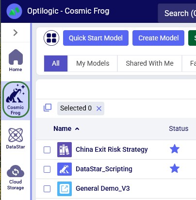
When logged into the Optilogic platform, you can open Cosmic Frog by clicking on its icon in the list of applications on the left. Note that the order of the applications may be different in your list so you may need to scroll down:
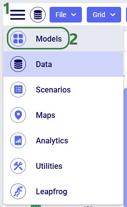
After opening Cosmic Frog, the model manager will typically be the active module. However, if you have been working in a specific model in Cosmic Frog previously, it may immediately open that model with its Data module being the active module. In that case, you can open the Model Manager from within Cosmic Frog by clicking on the icon with 3 horizontal bars at the left top to open the Module Menu, then select Models:
The Model Manager screen displays a table or grid of your existing models along with high level details such as name, status, and last modified date. This view is designed to give you immediate insight into your model library. The following screenshot shows at a high level the different features of the model manager. Each feature will be explained in more detail in subsequent sections of this documentation:
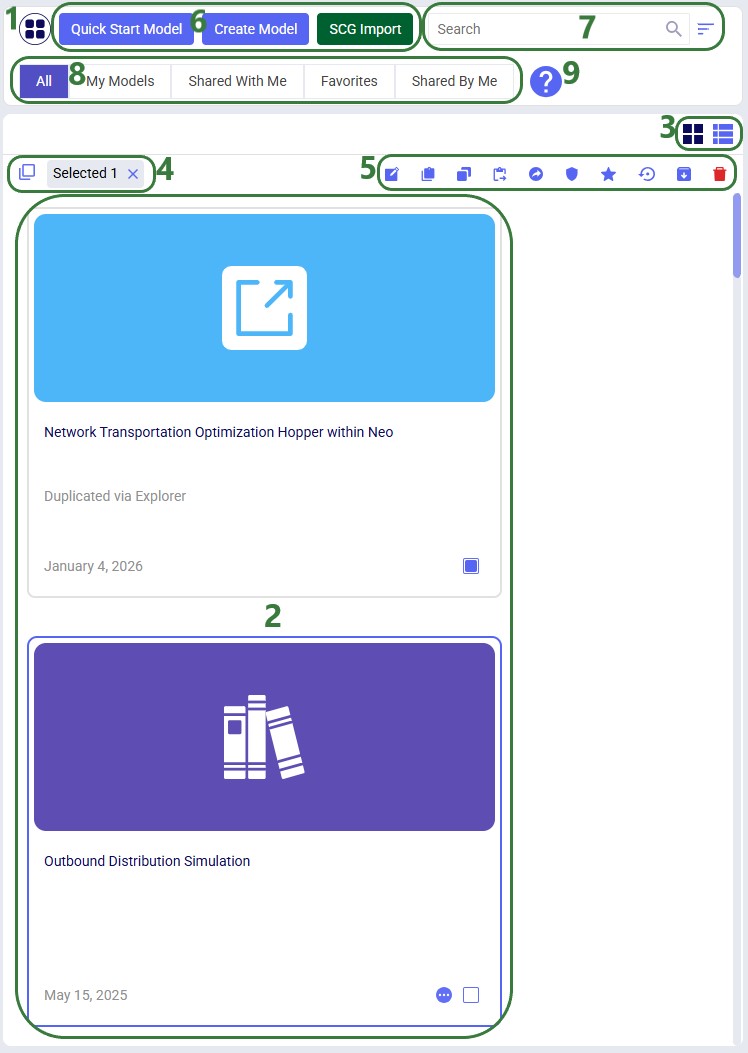
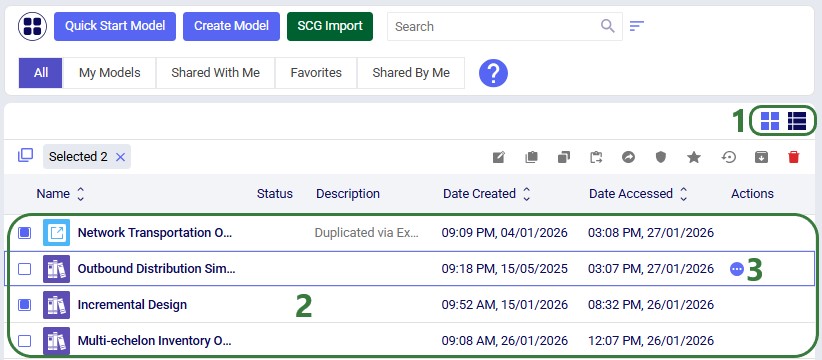
In the following screenshot we have switched from card view to list view:
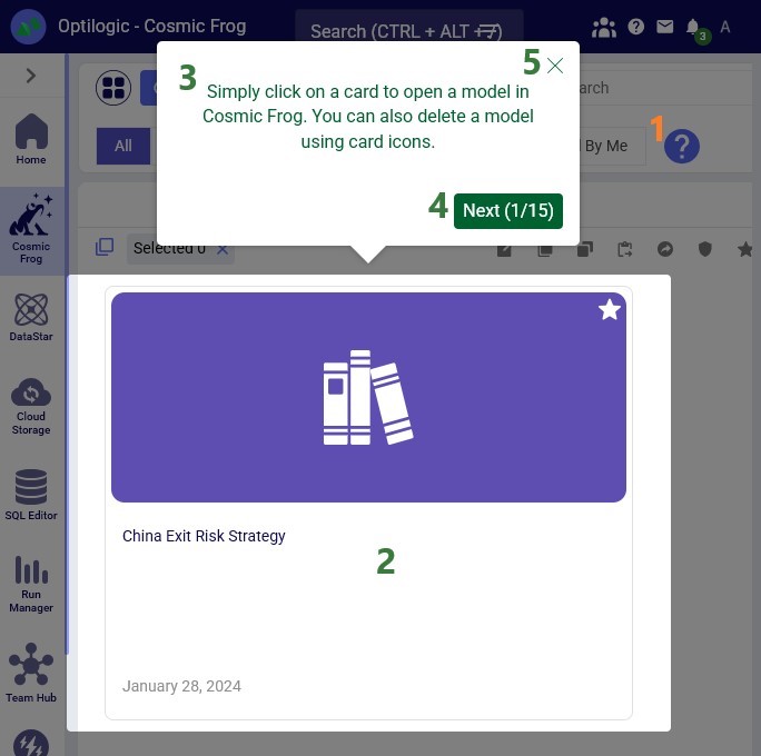
The Help & Hints area provides contextual guidance to help users understand the purpose of the Model Manager and how to use it effectively. These hints are especially useful for new users:
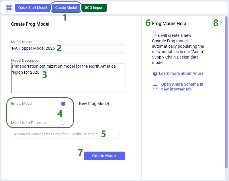
From the Model Manager there are a few options to create a new Cosmic Frog model, which will be covered in this section. We will start with the option from which new empty models as well as copies from Resource Library models can be created:
Another option to create a new model is to create one with tables populated from an Excel template, click on the Quick Start Model button to open the Create Quick Start Model form:
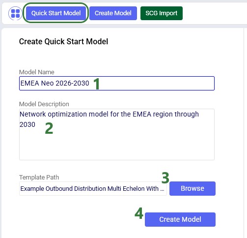
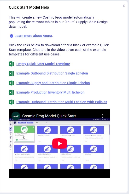
Note that for this option there is help available on the right-hand side of the form too, including example Excel template files, which can be downloaded to function as a starting point to overwrite with your own data. A video on this Quick Start option can be accessed from here too:
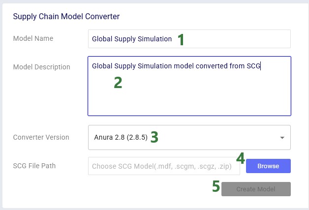
Finally, users also have the option to convert their Supply Chain Guru (SCG) models to a Cosmic Frog model. After clicking on the SCG Import button, the following Supply Chain Model Converter form comes up:
As your model library grows, search, sort, and filter tools help you quickly locate the models you need. The following screenshot shows the use of the search box and the available sort options:
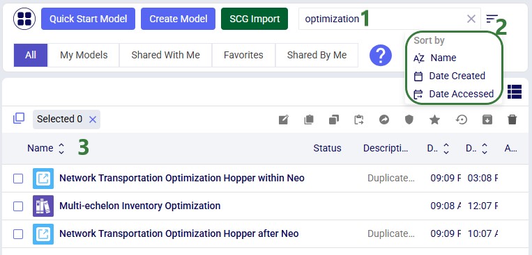
Standard filters to reduce the list of models to those of interest are also available:
To learn more about sharing models, please see this "Model Sharing & Backups for Multi-User Collaboration in Cosmic Frog" help center article.
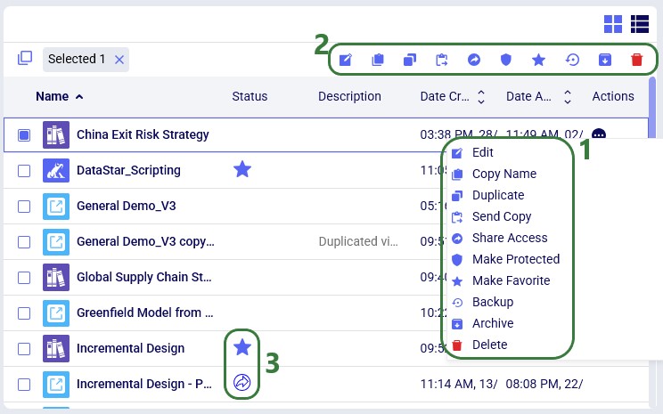
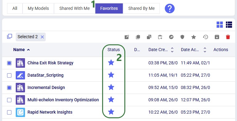
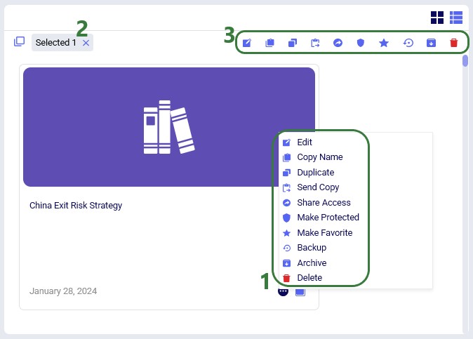
The Model Manager provides comprehensive model management capabilities through both the action toolbar and context menus. The first 2 screenshots in this section show these in card view, while the last screenshot shows the options while in list view:
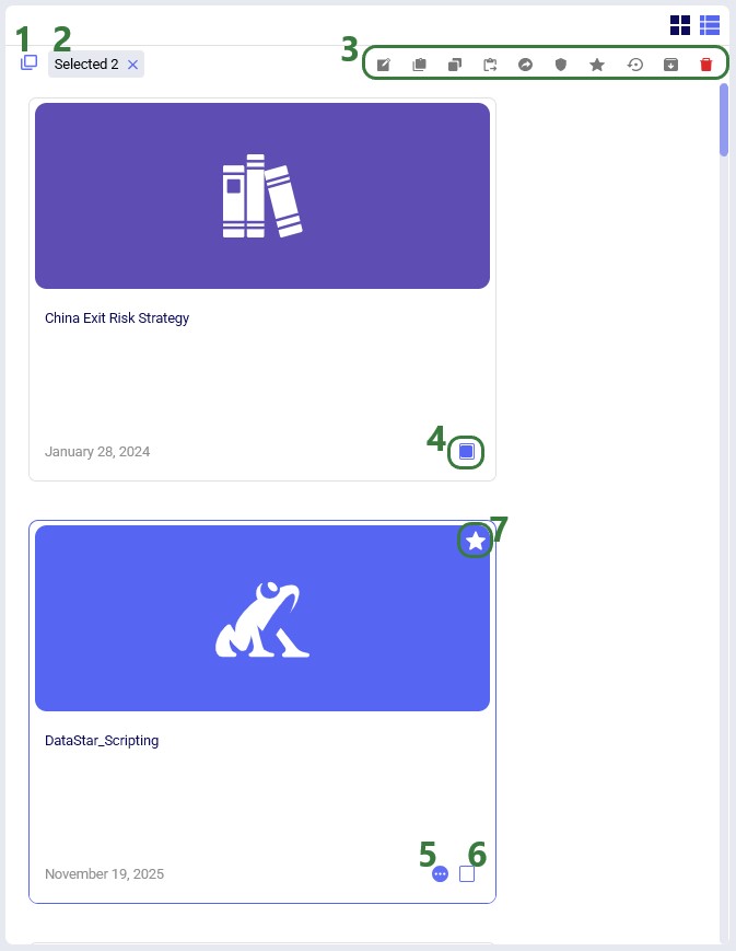
The model management actions available from the toolbar and from the context menu of a model in card view are shown in this next screenshot:
Lastly, the next screenshot shows the Model Management Actions while in list view: