Optilogic introduces the Lumina Tariff Optimizer – a powerful optimization engine that empowers companies to reoptimize supply chains in real-time to reduce the effects of tariffs. It provides instant clarity on today’s evolving tariff landscape, uncovers supply chain impacts, and recommends actions to stay ahead – now and into the future.
Manufacturers, distributors, and retailers around the world are faced with an enormous task trying to keep up with changing tariff policies and their supply chain impact. With Optilogic’s Lumina Tariff Optimizer, companies can illuminate their path forward by proactively designing tariff mitigation strategies that automatically consider the latest tariff rates.
With Lumina Tariff Optimizer, Optilogic users can stay ahead of tariff policy and answer critical questions to take swift action:
The following 7-minute video gives a great overview of the Lumina Tariff Optimizer tools:
Optilogic’s Lumina Tariff Optimization engine can be leveraged by modelers within Cosmic Frog or be leveraged within a Cosmic Frog for Excel app for other stakeholders across the business to evaluate the tariff impact to their end-to-end supply chain. Optilogic enables users to get started quickly with Lumina with several items in the Resource Library that include:
This documentation will cover each of these Lumina Tariff Optimizer tools, in the same order as listed above.
The first tool in the Lumina Tariff Optimizer toolset is the Tariffs example model which users can copy to their own account from the Resource Library. We will walk through this model, covering inputs and outputs, with emphasis on how to specify tariffs and their impact on the optimal solution when running network optimization (using the Neo engine) on the scenarios in the model.
Let us start by looking at the map of the Tariffs model, which is showing the model locations and flows for the Baseline scenario:
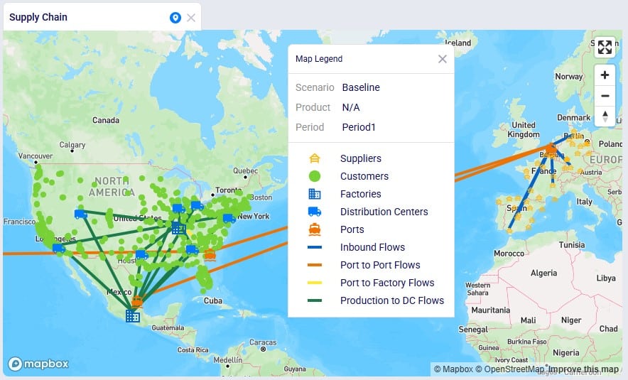
This model consists of the following sites:
Next, we will have a look at the Products table:

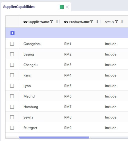
As mentioned above, raw materials RM1, RM2, and RM3 are supplied by Chinese suppliers and the others 6 raw materials by European suppliers, which we can confirm by looking at the Supplier Capabilities input table:
The Bills Of Materials input table shows that each finished good takes 3 of the Raw Materials to be manufactured; the Quantity field indicates how much of each is needed to create 1 unit of finished good:

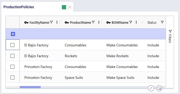
Looking at the Production Policies input table, we see that both the US and Mexico factory can produce Consumables, but Rockets are only manufactured in Mexico and Space Suits only in the US:
To understand the outputs later, we also need to briefly cover the Flow Constraints input table, which shows that the El Bajio Factory in Mexico can at a maximum ship out 3.5M units of finished goods (over all products and the model horizon together):

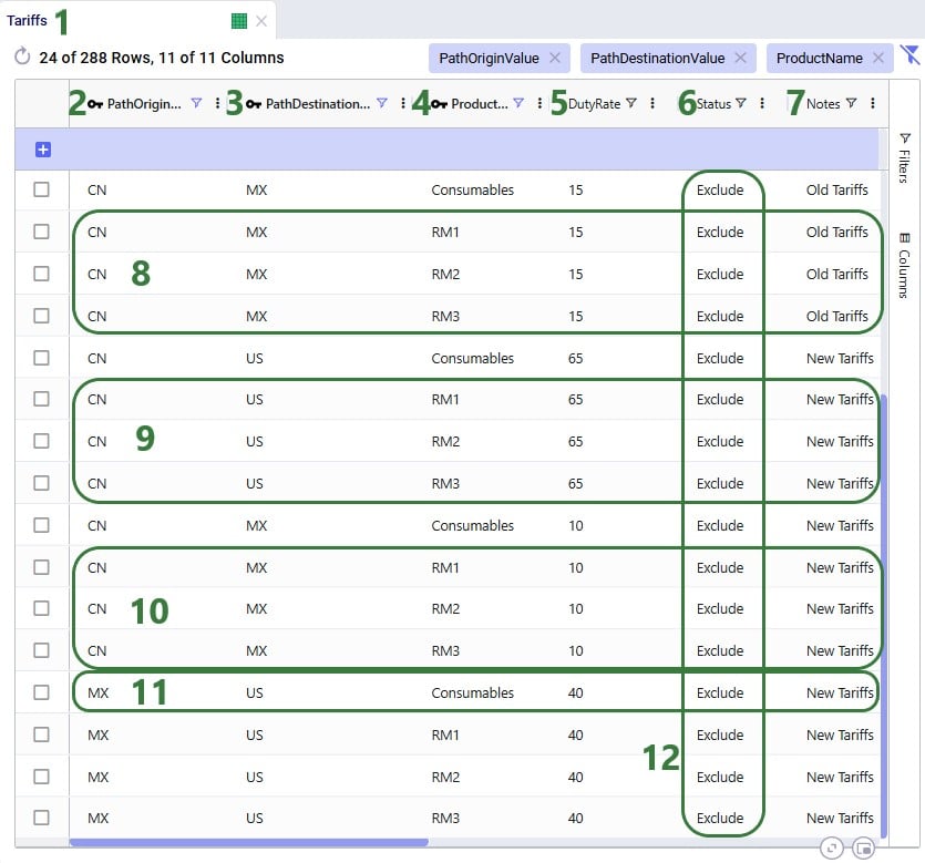
To enter tariffs and take them into account in a network optimization (Neo) run, users need to populate the new Tariffs input table:
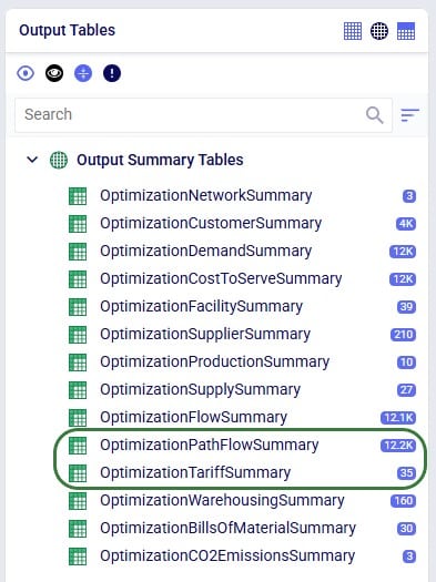
There are also 2 new Neo output tables that will be populated when tariffs are included in the model, the Optimization Path Flow Summary and the Optimization Tariff Summary tables:
Tariffs can be specified at multiple levels in Cosmic Frog, so users can choose the one that fits their modeling needs and available data best:
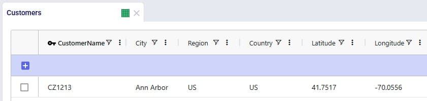
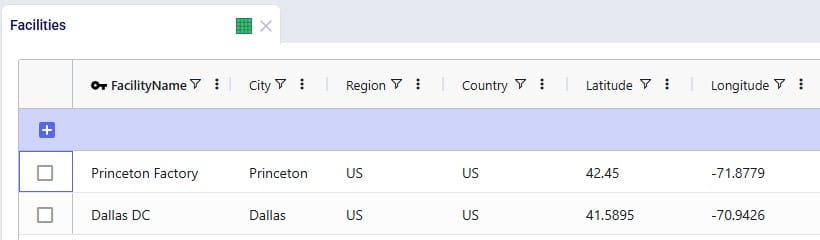
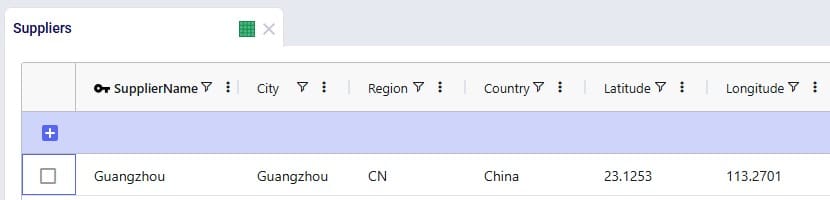
In order to model tariffs from/to a region or country, these fields need to be populated in the Customers, Facilities, and Suppliers tables:

In the Tariffs input table, all path origin location (furthest upstream) – path destination location (furthest downstream) – product combinations to which tariffs need to be applied are captured. There can be any number of echelons in between the path origin location and path destination location where the product flows through. Consider the following path that a raw material takes:

The raw material is manufactured/supplied from China (the path origin), it then flows through a location in Vietnam, then through a location in Mexico, before ending its path in the USA (the path destination, where it is consumed when manufacturing a finished good). In this case the tariff that is set up for this raw material with path origin = China, and path destination = USA will be applied. The tariff will be applied to the segment of the path where the product arrives in the region / country of its final destination. In the example here, that is on last leg (/lane / segment) of the path, e.g. on the Mexico to USA lane.
If we have a raw material that takes the same initial path, except it ends in Mexico to be consumed in a finished good, then the tariff that is set up for this raw material with path origin = China and path destination = Mexico will be applied. To continue from this example: then if this finished good manufactured in Mexico is shipped to the US and sold there, and if there is a path with a tariff set up from Mexico to USA for the finished good, then that tariff will be applied (path origin = Mexico, path destination = USA). I.e. in this last example the entire path is just the 1 segment between Mexico and USA.
So, now we will look how this can be set up in the Tariffs input table:
Please note:
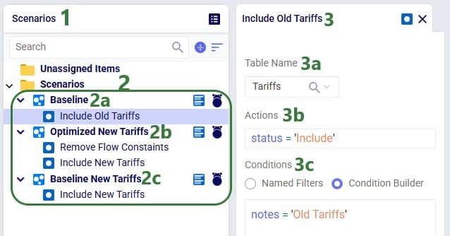
Three scenarios were run in the Tariffs example model:
Now, we will look at the outputs for these 3 scenarios, first at a higher level and later on, we will dig into some details of how the tariff costs are calculated as well.
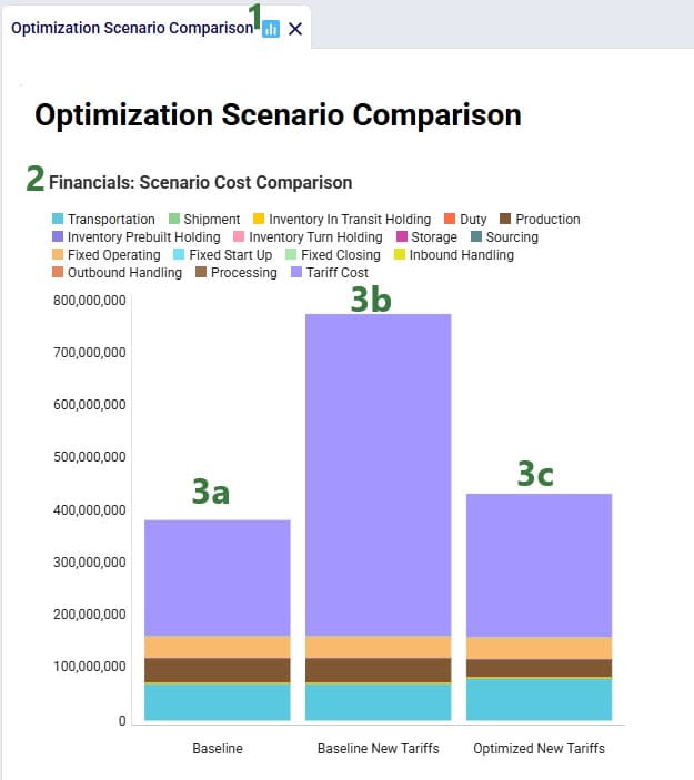
The Financials stacked bar chart in the standard Optimization Scenario Comparison dashboard in the Analytics module of Cosmic Frog can be used to compare all costs for all 3 scenarios in 1 graph:
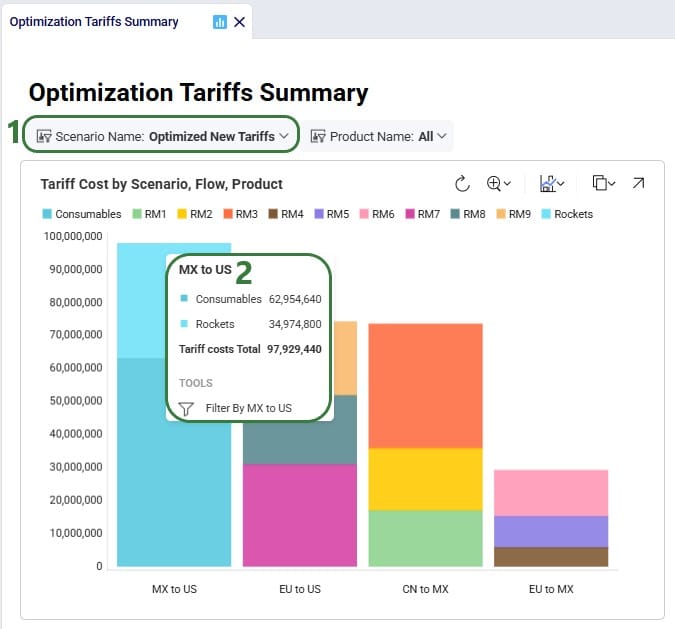
To compare the Tariffs by path origin – path destination and product, a new “Optimization Tariffs Summary” dashboard was created. We will look at the Baseline New Tariffs scenario first, and the Optimized New Tariffs scenario next:
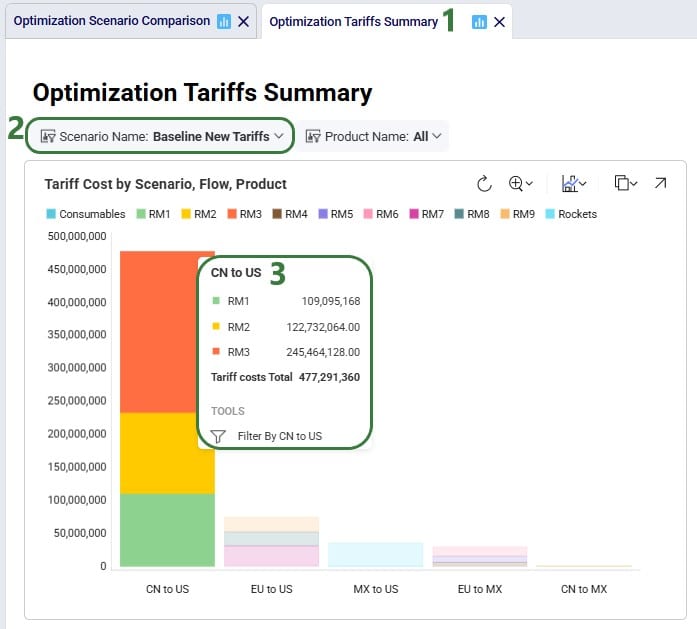
Note that in the Appendix it is explained how this chart can be created.
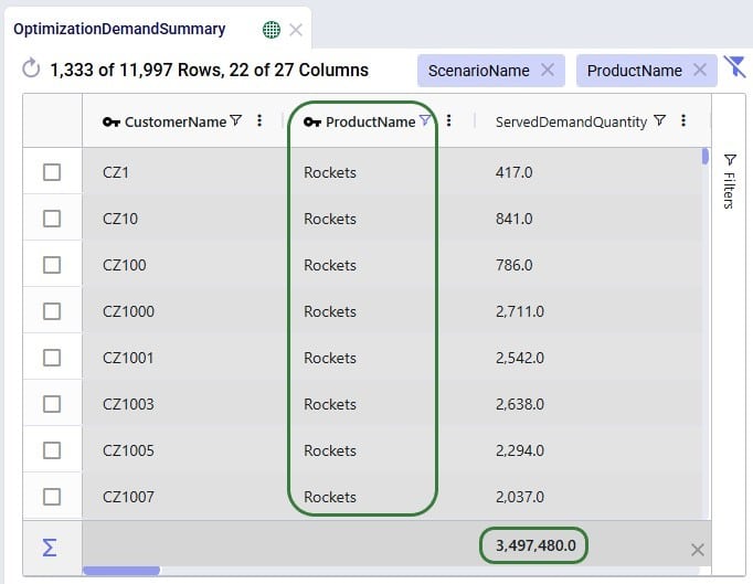
Next, we will take a closer look at some more detailed outputs. Starting with how much demand there is in the model for Rockets and Consumables, the 2 finished goods the Mexican factory in El Bajio can manufacture. The next screenshot shows the Optimization Demand Summary network optimization output table, filtered for Rockets and with a summation aggregation applied to it to show the total demand for Rockets at the bottom of the grid:
Next, we change the filter to look at the Consumables product:

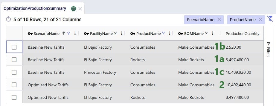
In conclusion: the demand for Rockets is nearly 3.5M units and for Consumables nearly 10.5M. Rockets can only be produced in Mexico whereas Consumables can be produced by both factories. From the charts above we suspected a shift in production from US to Mexico for the Consumables finished good in the Optimized New Tariffs scenario, which we can confirm by looking at the Optimization Production Summary output table:
Since the production of Consumables requires raw materials RM1, RM2, and RM3, we expect to see the above production quantities for Consumables to be reflected in the amount of these raw materials that was moved from the suppliers in China to the US vs to Mexico. We can see this in the Optimization Flow Summary network optimization output table, which is filtered for the 2 scenarios with new tariffs, Port to Port lanes, and these 3 raw materials:

The custom Optimization Tariff Summary and Optimization Path Flow Summary output tables are automatically generated after running a network optimization on a model with a populated Tariffs table. The first of these 2 is shown in the next screenshot where we have filtered out the raw materials RM1, RM2, and RM3 again, plus also the Consumables finished good for the 2 scenarios that use the new tariffs:

Where the Optimization Tariff Summary output table summarizes the tariffs at the scenario - path origin – path destination – product level, the Optimization Path Flow Summary output table gives some more detail around the whole path, and on which segments the tariffs are applied. The next 2 screenshots show 6 records of this output table for the Tariffs example model:
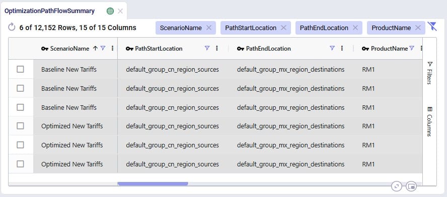
For the 2 scenarios that use the new tariffs, records are filtered out for raw material RM1 where the Path Start Location represents the CN region and the Path End Location represents the MX region. These Path Start and End Locations are automatically generated based on the Path Origin Property and Value and Destination Property and Value set in the Tariffs input table. Scrolling right for these 6 records:
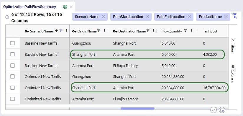
We see that the path for RM1 is the same in both scenarios: originate at location Guangzhou in China, moved to Shanghai Port (CN), from Shanghai Port moved to Altamira Port (MX), and from Altamira Port moved to the El Bajio Factory (MX). The calculations of the Tariff Cost based on the Flow Quantity are the same as explained above, and we see that the tariffs are applied on the second segment where the product arrives in the region / country of its final destination.
Wondering where to go from here? If you are wanting to start using tariffs in your own models, but are not exactly sure where to start, please see the “Cosmic Frog Utilities to Create the Tariffs Table” section further below, which also includes step-by-step instructions based on what data you have available.
In the next section, we will first discuss how quick sensitivity analyses around tariffs can be run using a Cosmic Frog for Excel App.
To enable Cosmic Frog users, and also managers and executives with no or limited knowledge of Cosmic Frog, to run quick sensitivity scenarios around changing tariffs, Optilogic has developed an Excel Application for this specific purpose. Users can connect to their Cosmic Frog model that contains a populated Tariffs input table and indicate which tariffs to increase/decrease by how much, run network optimization with these changed tariffs, and review the optimization tariff summary output table, all in 1 Excel workbook. Users can download this application and related files from the Resource Library.
The following represents a typical workflow when using the Tariffs Rapid Optimizer application:

For users to take advantage of the power of the Lumina Tariff Optimizer they will want to create their own network optimization model which includes a populated Tariffs input table (see also the “Tariffs Model – Tariffs Table” section earlier in this documentation). Depending on the data available to the user, populating the Tariffs input table can be a straightforward task or a difficult one in case no or little data around tariffs is known/available within the organization. Optilogic has developed 3 utilities to help users with this task. The utilities are available from within Cosmic Frog, which will be covered in this section of the documentation, and they are also available through the Cosmic Frog for Excel Tariffs Builder App, which will be covered in the next section. Here follows a short description of each utility, they will each be covered in more detail later in this section:
In Cosmic Frog, they are accessible from the Utilities module (click on the 3 horizontal bars icon at the top left in Cosmic Frog to open the Module menu drop-down and select Utilities):
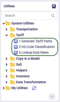
The utilities are listed under System Utilities > Tariff.
The latter 2 utilities hook into Avalara APIs, and users need to use / obtain their own Avalara API keys for each to be able to use these utilities from within Cosmic Frog or the Tariffs Builder Excel App.
The following list shows the recommended steps for users with varying levels of Tariffs data available to them from least to most data available (assuming an otherwise complete Cosmic Frog model has been built):
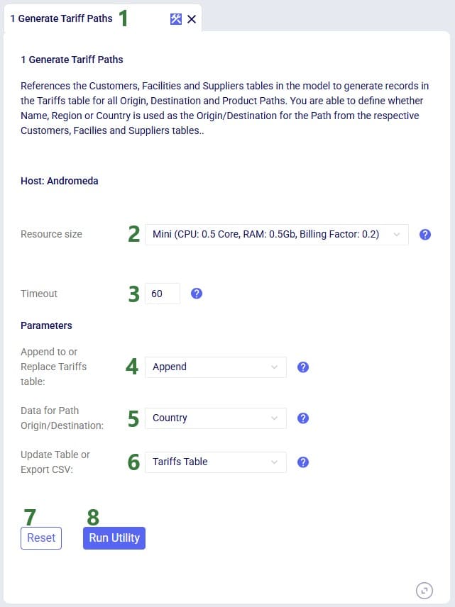
To populate the Tariffs table with all possible path origin – path destination – product combinations, based on the contents of the Transportation Policies input table, use this first utility:
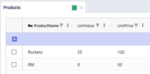
Consider a small model with 1 customer in the US, 2 facilities (1 DC and 1 factory) both in the US, 1 supplier in China, and 2 products (1 finished good and 1 component):
After running the 1 Generate Tariff Paths utility (using Region as the data to use for the path origin and path destination), the Tariffs table is generated and populated as shown in the next 2 screenshots:
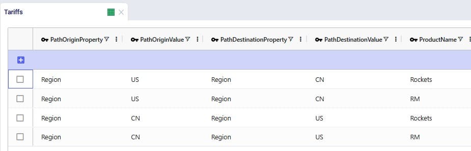
All combinations for path origin region, path destination region, and product have been added to the Tariffs table. Scrolling further right, we see the remaining fields of this table:
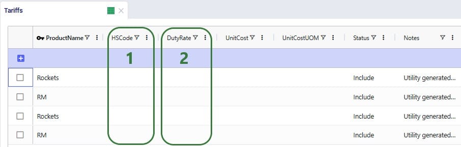
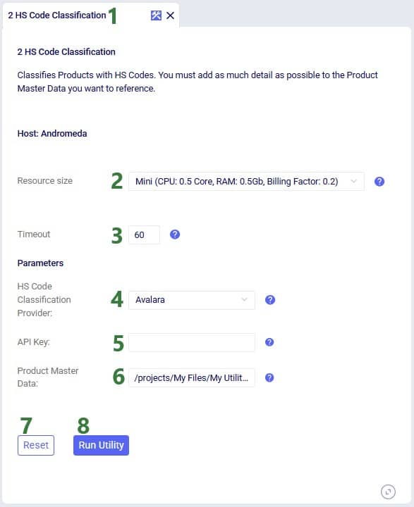
To update the HS Code field in the Tariffs table, we can use the second utility:
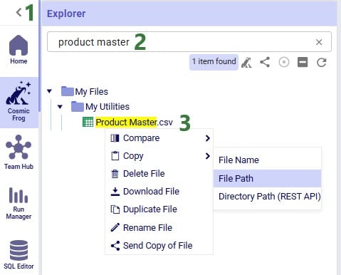
Users can find the full path of a file uploaded to their Optilogic account as follows:
The file containing the product master data needs to have the same columns as shown in the next screenshot:
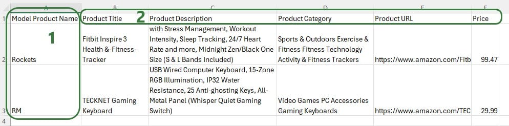
Note that columns B-F contain information of products that do not match the product name in Cosmic Frog as this is just an example to show how the utility works.
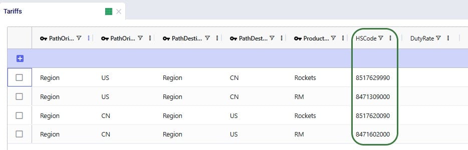
After running the 2 HS Code Classification utility, we see that the HS Code field in the Tariffs table is now populated:
To use the HS Code field to next look up duty rates we can use the third utility:
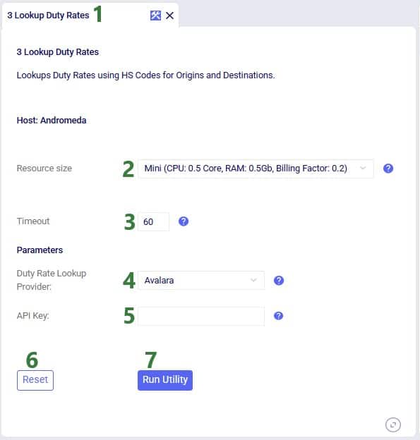
After running the 3 Lookup Duty Rates utility, we see that the Duty Rate field in the Tariffs table is now populated:
The raw output from the API is placed in the Duty Rate field and user needs to update this so that the field contains just a number representing the total duty rate. For the second record (US region to China region for product RM), the total duty rate is 35% (25% + 10%), and user needs to enter 35 in this field. For the third record (China region to US region for product Rockets), the duty rate is 27.5% (7.5% + 20%), and user needs to enter 27.5 in this field. For the fourth record (China region to US region for product RM), the total duty rate is 25%, and user needs to enter 25 in this field.
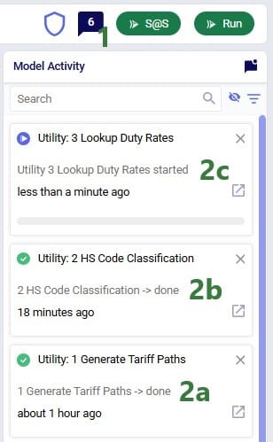
When running a utility in Cosmic Frog, user can track the progress in the Model Activity window:
The 3 utilities covered in the previous section to generate and populate the Tariffs input table are also made available in the Cosmic Frog for Excel Tariffs Builder App, which we will cover in this section. Users can download this application and related files from the Resource Library.
The following represents a typical workflow when using this Tariffs Builder application:
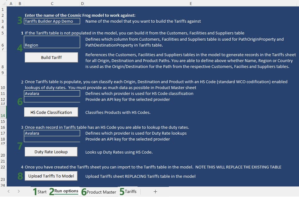
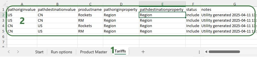
The next screenshot shows the Tariffs table after just running the Build Tariff workflow (bullet 4 in the list above):
The next screenshot shows the Product Master worksheet which contains the product information to be used by the HS Code Classification workflow, it needs to be in this format and users should enter as much product information in here as possible:
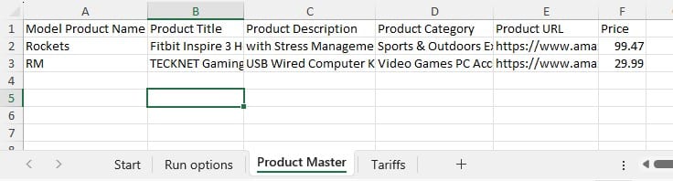
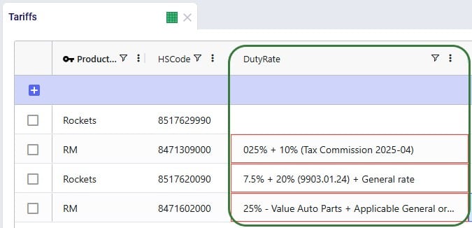
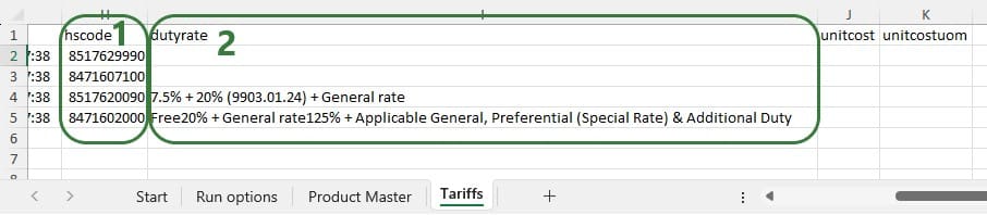
After also running the HS Code Classification and the Duty Rate Lookup workflows (bullets 6 and 7 in the list further above), we see that these fields are now also populated on the Tariffs worksheet:
We hope users feel empowered to take on the challenging task of incorporating tariffs into their optimization workflows. For any questions, please do not hesitate to contact Optilogic support on support@optilogic.com.
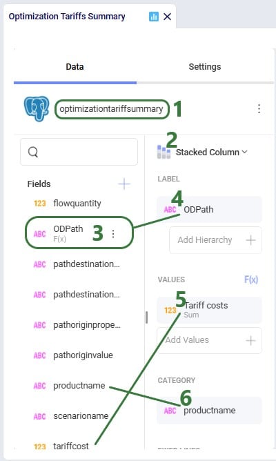
In this appendix we will show users how to create a stacked bar chart for each path origin – path destination pair, showing the tariff costs by product.
In the Analytics drop-down menu in the toolbar while in the Analytics module of Cosmic Frog, select New Dashboard, give it a name (e.g. Optimization Tariff Summary), then click on the blue Visualization button on the top right to create a new chart for the dashboard. In the New Visualization configuration form that comes up, type “tariff” in the Tables Search box, then check the box for the Optimization Tariff Summary table in the list, and click on Select Data.
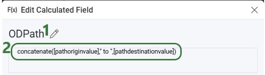
To create the OD Path calculated field, click on the plus icon at the top right of the Fields list and select Calculated Field which brings up the Edit Calculated Field configuration window:
Optilogic introduces the Lumina Tariff Optimizer – a powerful optimization engine that empowers companies to reoptimize supply chains in real-time to reduce the effects of tariffs. It provides instant clarity on today’s evolving tariff landscape, uncovers supply chain impacts, and recommends actions to stay ahead – now and into the future.
Manufacturers, distributors, and retailers around the world are faced with an enormous task trying to keep up with changing tariff policies and their supply chain impact. With Optilogic’s Lumina Tariff Optimizer, companies can illuminate their path forward by proactively designing tariff mitigation strategies that automatically consider the latest tariff rates.
With Lumina Tariff Optimizer, Optilogic users can stay ahead of tariff policy and answer critical questions to take swift action:
The following 7-minute video gives a great overview of the Lumina Tariff Optimizer tools:
Optilogic’s Lumina Tariff Optimization engine can be leveraged by modelers within Cosmic Frog or be leveraged within a Cosmic Frog for Excel app for other stakeholders across the business to evaluate the tariff impact to their end-to-end supply chain. Optilogic enables users to get started quickly with Lumina with several items in the Resource Library that include:
This documentation will cover each of these Lumina Tariff Optimizer tools, in the same order as listed above.
The first tool in the Lumina Tariff Optimizer toolset is the Tariffs example model which users can copy to their own account from the Resource Library. We will walk through this model, covering inputs and outputs, with emphasis on how to specify tariffs and their impact on the optimal solution when running network optimization (using the Neo engine) on the scenarios in the model.
Let us start by looking at the map of the Tariffs model, which is showing the model locations and flows for the Baseline scenario:
This model consists of the following sites:
Next, we will have a look at the Products table:
As mentioned above, raw materials RM1, RM2, and RM3 are supplied by Chinese suppliers and the others 6 raw materials by European suppliers, which we can confirm by looking at the Supplier Capabilities input table:
The Bills Of Materials input table shows that each finished good takes 3 of the Raw Materials to be manufactured; the Quantity field indicates how much of each is needed to create 1 unit of finished good:
Looking at the Production Policies input table, we see that both the US and Mexico factory can produce Consumables, but Rockets are only manufactured in Mexico and Space Suits only in the US:
To understand the outputs later, we also need to briefly cover the Flow Constraints input table, which shows that the El Bajio Factory in Mexico can at a maximum ship out 3.5M units of finished goods (over all products and the model horizon together):
To enter tariffs and take them into account in a network optimization (Neo) run, users need to populate the new Tariffs input table:
There are also 2 new Neo output tables that will be populated when tariffs are included in the model, the Optimization Path Flow Summary and the Optimization Tariff Summary tables:
Tariffs can be specified at multiple levels in Cosmic Frog, so users can choose the one that fits their modeling needs and available data best:
In order to model tariffs from/to a region or country, these fields need to be populated in the Customers, Facilities, and Suppliers tables:
In the Tariffs input table, all path origin location (furthest upstream) – path destination location (furthest downstream) – product combinations to which tariffs need to be applied are captured. There can be any number of echelons in between the path origin location and path destination location where the product flows through. Consider the following path that a raw material takes:
The raw material is manufactured/supplied from China (the path origin), it then flows through a location in Vietnam, then through a location in Mexico, before ending its path in the USA (the path destination, where it is consumed when manufacturing a finished good). In this case the tariff that is set up for this raw material with path origin = China, and path destination = USA will be applied. The tariff will be applied to the segment of the path where the product arrives in the region / country of its final destination. In the example here, that is on last leg (/lane / segment) of the path, e.g. on the Mexico to USA lane.
If we have a raw material that takes the same initial path, except it ends in Mexico to be consumed in a finished good, then the tariff that is set up for this raw material with path origin = China and path destination = Mexico will be applied. To continue from this example: then if this finished good manufactured in Mexico is shipped to the US and sold there, and if there is a path with a tariff set up from Mexico to USA for the finished good, then that tariff will be applied (path origin = Mexico, path destination = USA). I.e. in this last example the entire path is just the 1 segment between Mexico and USA.
So, now we will look how this can be set up in the Tariffs input table:
Please note:
Three scenarios were run in the Tariffs example model:
Now, we will look at the outputs for these 3 scenarios, first at a higher level and later on, we will dig into some details of how the tariff costs are calculated as well.
The Financials stacked bar chart in the standard Optimization Scenario Comparison dashboard in the Analytics module of Cosmic Frog can be used to compare all costs for all 3 scenarios in 1 graph:
To compare the Tariffs by path origin – path destination and product, a new “Optimization Tariffs Summary” dashboard was created. We will look at the Baseline New Tariffs scenario first, and the Optimized New Tariffs scenario next:
Note that in the Appendix it is explained how this chart can be created.
Next, we will take a closer look at some more detailed outputs. Starting with how much demand there is in the model for Rockets and Consumables, the 2 finished goods the Mexican factory in El Bajio can manufacture. The next screenshot shows the Optimization Demand Summary network optimization output table, filtered for Rockets and with a summation aggregation applied to it to show the total demand for Rockets at the bottom of the grid:
Next, we change the filter to look at the Consumables product:
In conclusion: the demand for Rockets is nearly 3.5M units and for Consumables nearly 10.5M. Rockets can only be produced in Mexico whereas Consumables can be produced by both factories. From the charts above we suspected a shift in production from US to Mexico for the Consumables finished good in the Optimized New Tariffs scenario, which we can confirm by looking at the Optimization Production Summary output table:
Since the production of Consumables requires raw materials RM1, RM2, and RM3, we expect to see the above production quantities for Consumables to be reflected in the amount of these raw materials that was moved from the suppliers in China to the US vs to Mexico. We can see this in the Optimization Flow Summary network optimization output table, which is filtered for the 2 scenarios with new tariffs, Port to Port lanes, and these 3 raw materials:
The custom Optimization Tariff Summary and Optimization Path Flow Summary output tables are automatically generated after running a network optimization on a model with a populated Tariffs table. The first of these 2 is shown in the next screenshot where we have filtered out the raw materials RM1, RM2, and RM3 again, plus also the Consumables finished good for the 2 scenarios that use the new tariffs:
Where the Optimization Tariff Summary output table summarizes the tariffs at the scenario - path origin – path destination – product level, the Optimization Path Flow Summary output table gives some more detail around the whole path, and on which segments the tariffs are applied. The next 2 screenshots show 6 records of this output table for the Tariffs example model:
For the 2 scenarios that use the new tariffs, records are filtered out for raw material RM1 where the Path Start Location represents the CN region and the Path End Location represents the MX region. These Path Start and End Locations are automatically generated based on the Path Origin Property and Value and Destination Property and Value set in the Tariffs input table. Scrolling right for these 6 records:
We see that the path for RM1 is the same in both scenarios: originate at location Guangzhou in China, moved to Shanghai Port (CN), from Shanghai Port moved to Altamira Port (MX), and from Altamira Port moved to the El Bajio Factory (MX). The calculations of the Tariff Cost based on the Flow Quantity are the same as explained above, and we see that the tariffs are applied on the second segment where the product arrives in the region / country of its final destination.
Wondering where to go from here? If you are wanting to start using tariffs in your own models, but are not exactly sure where to start, please see the “Cosmic Frog Utilities to Create the Tariffs Table” section further below, which also includes step-by-step instructions based on what data you have available.
In the next section, we will first discuss how quick sensitivity analyses around tariffs can be run using a Cosmic Frog for Excel App.
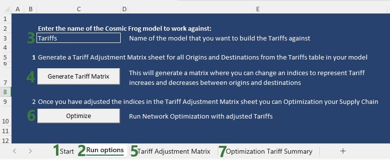
To enable Cosmic Frog users, and also managers and executives with no or limited knowledge of Cosmic Frog, to run quick sensitivity scenarios around changing tariffs, Optilogic has developed an Excel Application for this specific purpose. Users can connect to their Cosmic Frog model that contains a populated Tariffs input table and indicate which tariffs to increase/decrease by how much, run network optimization with these changed tariffs, and review the optimization tariff summary output table, all in 1 Excel workbook. Users can download this application and related files from the Resource Library.
The following represents a typical workflow when using the Tariffs Rapid Optimizer application:
For users to take advantage of the power of the Lumina Tariff Optimizer they will want to create their own network optimization model which includes a populated Tariffs input table (see also the “Tariffs Model – Tariffs Table” section earlier in this documentation). Depending on the data available to the user, populating the Tariffs input table can be a straightforward task or a difficult one in case no or little data around tariffs is known/available within the organization. Optilogic has developed 3 utilities to help users with this task. The utilities are available from within Cosmic Frog, which will be covered in this section of the documentation, and they are also available through the Cosmic Frog for Excel Tariffs Builder App, which will be covered in the next section. Here follows a short description of each utility, they will each be covered in more detail later in this section:
In Cosmic Frog, they are accessible from the Utilities module (click on the 3 horizontal bars icon at the top left in Cosmic Frog to open the Module menu drop-down and select Utilities):
The utilities are listed under System Utilities > Tariff.
The latter 2 utilities hook into Avalara APIs, and users need to use / obtain their own Avalara API keys for each to be able to use these utilities from within Cosmic Frog or the Tariffs Builder Excel App.
The following list shows the recommended steps for users with varying levels of Tariffs data available to them from least to most data available (assuming an otherwise complete Cosmic Frog model has been built):
To populate the Tariffs table with all possible path origin – path destination – product combinations, based on the contents of the Transportation Policies input table, use this first utility:
Consider a small model with 1 customer in the US, 2 facilities (1 DC and 1 factory) both in the US, 1 supplier in China, and 2 products (1 finished good and 1 component):
After running the 1 Generate Tariff Paths utility (using Region as the data to use for the path origin and path destination), the Tariffs table is generated and populated as shown in the next 2 screenshots:
All combinations for path origin region, path destination region, and product have been added to the Tariffs table. Scrolling further right, we see the remaining fields of this table:
To update the HS Code field in the Tariffs table, we can use the second utility:
Users can find the full path of a file uploaded to their Optilogic account as follows:
The file containing the product master data needs to have the same columns as shown in the next screenshot:
Note that columns B-F contain information of products that do not match the product name in Cosmic Frog as this is just an example to show how the utility works.
After running the 2 HS Code Classification utility, we see that the HS Code field in the Tariffs table is now populated:
To use the HS Code field to next look up duty rates we can use the third utility:
After running the 3 Lookup Duty Rates utility, we see that the Duty Rate field in the Tariffs table is now populated:
The raw output from the API is placed in the Duty Rate field and user needs to update this so that the field contains just a number representing the total duty rate. For the second record (US region to China region for product RM), the total duty rate is 35% (25% + 10%), and user needs to enter 35 in this field. For the third record (China region to US region for product Rockets), the duty rate is 27.5% (7.5% + 20%), and user needs to enter 27.5 in this field. For the fourth record (China region to US region for product RM), the total duty rate is 25%, and user needs to enter 25 in this field.
When running a utility in Cosmic Frog, user can track the progress in the Model Activity window:
The 3 utilities covered in the previous section to generate and populate the Tariffs input table are also made available in the Cosmic Frog for Excel Tariffs Builder App, which we will cover in this section. Users can download this application and related files from the Resource Library.
The following represents a typical workflow when using this Tariffs Builder application:
The next screenshot shows the Tariffs table after just running the Build Tariff workflow (bullet 4 in the list above):
The next screenshot shows the Product Master worksheet which contains the product information to be used by the HS Code Classification workflow, it needs to be in this format and users should enter as much product information in here as possible:
After also running the HS Code Classification and the Duty Rate Lookup workflows (bullets 6 and 7 in the list further above), we see that these fields are now also populated on the Tariffs worksheet:
We hope users feel empowered to take on the challenging task of incorporating tariffs into their optimization workflows. For any questions, please do not hesitate to contact Optilogic support on support@optilogic.com.
In this appendix we will show users how to create a stacked bar chart for each path origin – path destination pair, showing the tariff costs by product.
In the Analytics drop-down menu in the toolbar while in the Analytics module of Cosmic Frog, select New Dashboard, give it a name (e.g. Optimization Tariff Summary), then click on the blue Visualization button on the top right to create a new chart for the dashboard. In the New Visualization configuration form that comes up, type “tariff” in the Tables Search box, then check the box for the Optimization Tariff Summary table in the list, and click on Select Data.
To create the OD Path calculated field, click on the plus icon at the top right of the Fields list and select Calculated Field which brings up the Edit Calculated Field configuration window: