For various reasons, many supply chains need to deal with returns. This can for example be due to packaging materials coming back to be reused at plants or DCs, retail customers returning finished goods that they are not happy with, defective products, etc. Previously, these returns could mostly be modelled within Cosmic Frog NEO (Network Optimization) models by using some tricks and workarounds. But with the latest Cosmic Frog release, returns are now supported natively, so that the reuse, repurposing, or recycling of these retuned products to help companies reduce costs, minimize waste, and improve overall supply chain efficiency can be taken into account easily.
This documentation will first provide an overview of how returns work in a Cosmic Frog model and then walk through an example model of a retailer which includes modelling the returns of finished goods. The appendix details all the new returns-related fields in several new tables and some of the existing tables.
When modelling returns in Cosmic Frog:
Users need to use 2 new input tables to set up returns:
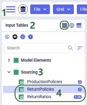
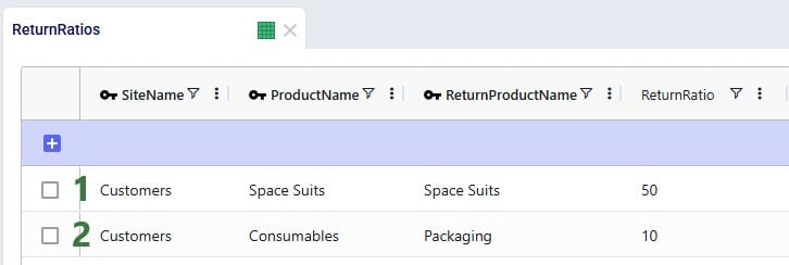
The Return Ratios table contains the information on how much return-product is returned for a certain amount of product delivered to a certain destination:
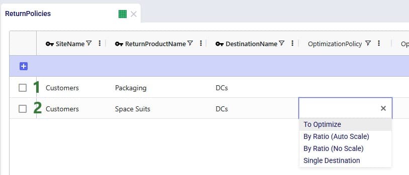
The Return Policies table is used to indicate where returned products need to go to and the rules around multiple possible destinations. Optionally, costs can be associated with the returns here and a maximum distance allowed for returns can be entered on this table too.
Note that both these tables have Status and Notes fields (not shown in the screenshots), like most Cosmic Frog input tables have. These are often used for scenario creation where the Status is set to Exclude in the table itself and changed to Include in select scenarios based on text in the Notes field.
All columns on these 2 returns-related input table are explained in more detail in the appendix.
In addition to populating the Return Policies and Return Ratios tables, users need to be aware that additional model structure needed for the returned products may need to be put in place:
The Optimization Return Summary output table is a new output table that will be generated for Neo runs if returns are included in the modelling:
This table and all its fields are explained in detail in the appendix.
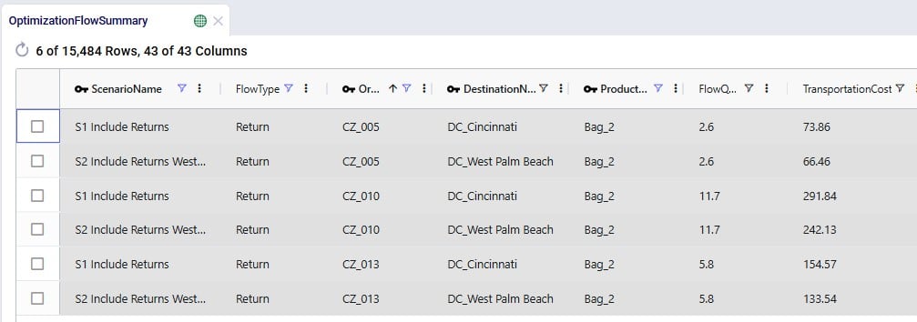
The Optimization Flow Summary output table will contain additional records for models that include returns; they can be identified by filtering the Flow Type field for “Return”:
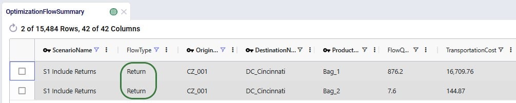
These 2 records show the return flows and associated transportation costs for the Bag_1 and Bag_2 products from CZ_001, going to DC_Cincinnati, that we saw in the Optimization Return Summary table screenshot above.
In addition to the new Optimization Return Summary output table, and new records of Flow Type = Return in the Optimization Flow Summary output table, following existing output tables now contain additional fields related to returns:
The example Returns model can be copied from the Resource Library to a user’s Optilogic account (see this help center article on how to use the Resource Library). It models the US supply chain of a fashion bag retailer. The model’s locations and flows both to customers and between DCs are shown in this screenshot (returns are not yet included here):
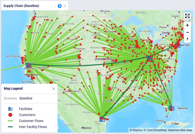
Historically, the retailer had 1 main DC in Cincinnati, Ohio, where all products were received and all 869 customers were fulfilled from. Over time, 4 secondary DCs were added based on Greenfield analysis, 2 bigger ones in Clovis, California, and Jersey City, New Jersey, and 2 smaller ones in West Palm Beach, Florida, and Las Lomas, Texas. These secondary DCs receive product from the Cincinnati DC and serve their own set of customers. The main DC in Cincinnati and the 2 bigger secondary DCs (Clovis, CA, and Jersey City, NJ) can handle returns currently: returns are received there and re-used to fulfill demand. However, until now, these returns had not been taken into account in the modelling. In this model we will explore following scenarios:
Other model features:
Please note that in this model the order of columns in the tables has sometimes been changed to put those containing data together on the left-hand side of the table. All columns are still present in the table but may be in a different position than you are used to. Columns can be reset to their default position by choosing “Reset Columns” from the menu that comes up when clicking on the icon with 3 vertical dots to the right of a column name.
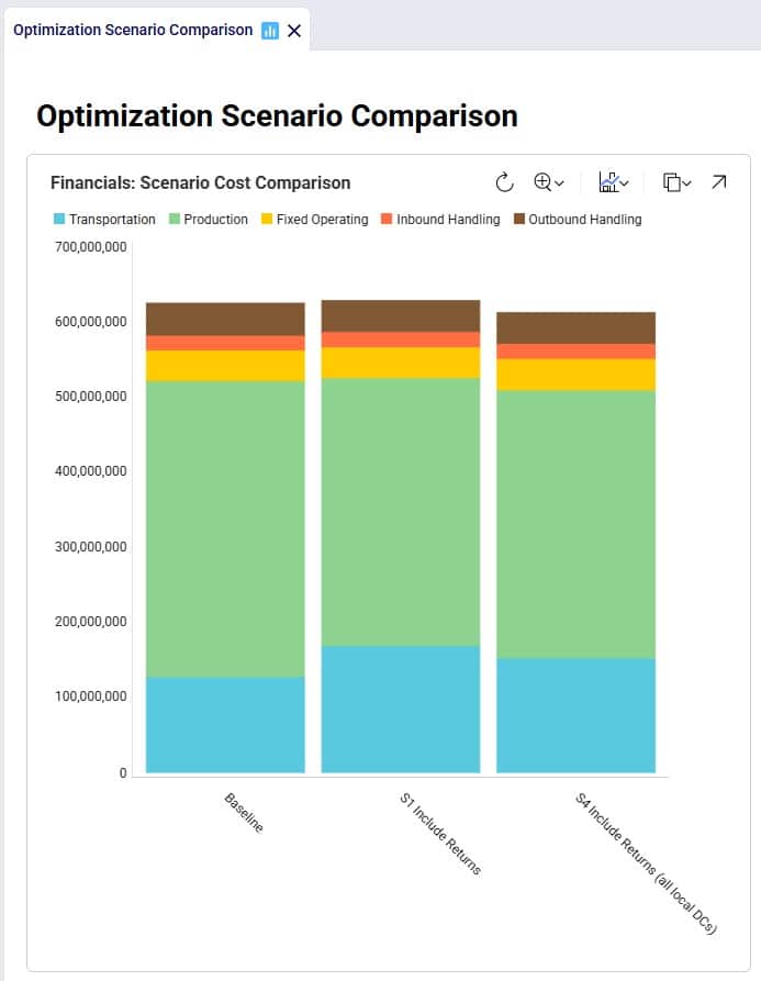
After running the baseline scenario (which does not include returns), we take a look at the Financials: Scenario Cost Comparison chart in the Optimization Scenario Comparison dashboard (in Cosmic Frog’s Analytics module):
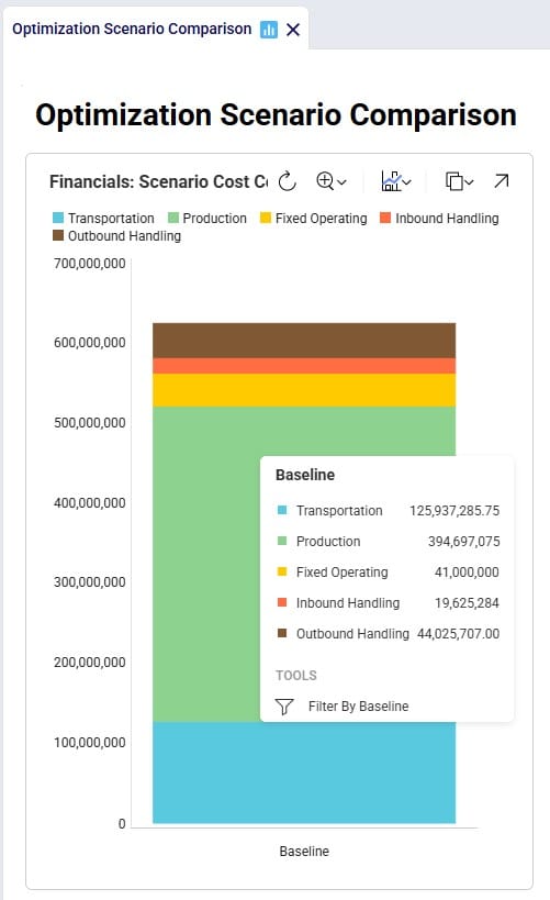
We see that the biggest cost currently is the production cost at 394.7M (= procurement of all product into Cincinnati), followed by transportation costs at 125.9M. The total supply chain cost of this scenario is 625.3M.
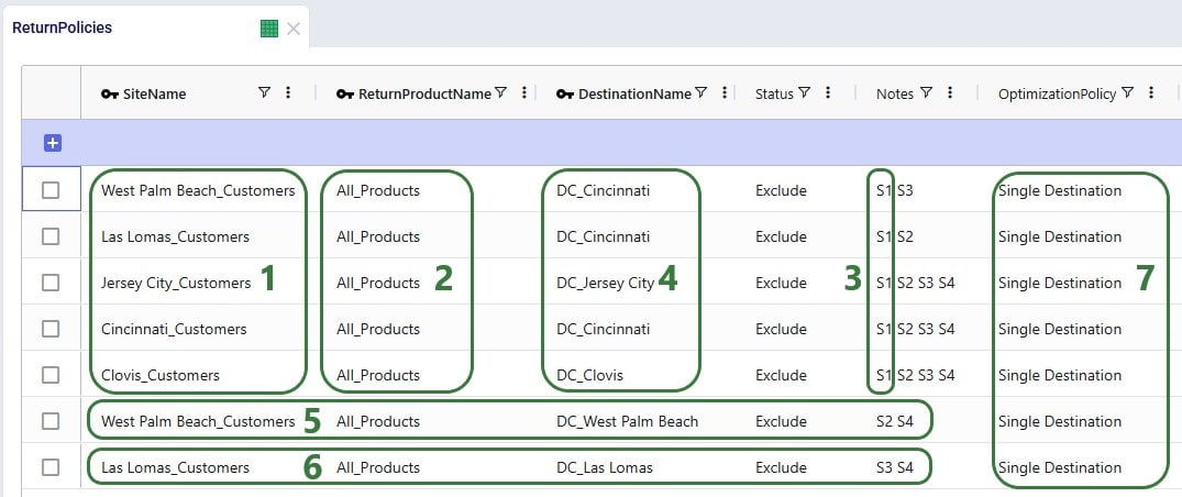
In this scenario we want to include how returns currently work: Cincinnati, Clovis, and Jersey City customers return their products to their local DCs whereas West Palm Beach and Las Lomas customers return their products to the main DC in Cincinnati. To set this up, we need to add records to the Return Policies, Return Ratios, and Transportation Policies input tables. To not change the Baseline scenario, all new records will be added with Status = Exclude, and the Notes field populated so it can be used to filter on in scenario items that change the Status to Include for subsets of records. Starting with the Return Policies table:
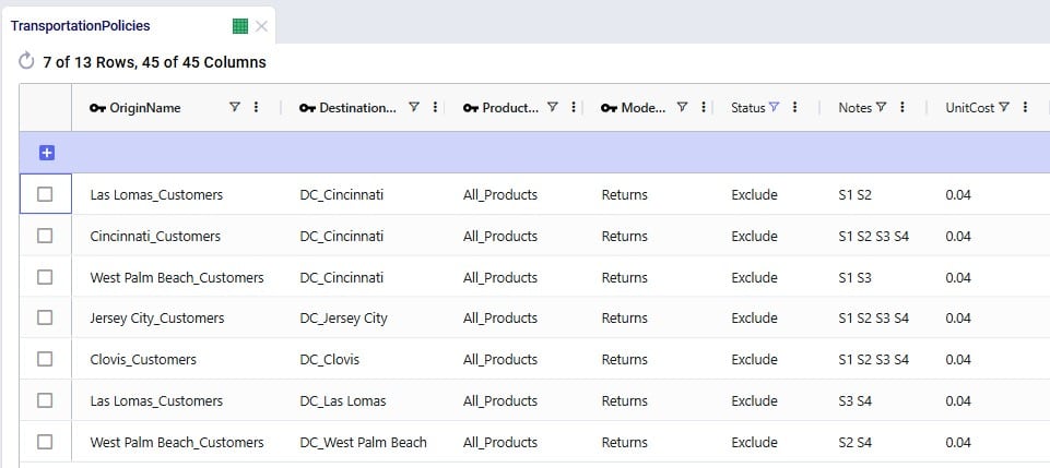
Next, we need to add records to the Transportation Policies table so that there is at least 1 lane available for each site-product-destination combination set up in the return policies table. For this example, we add records to the Transportation Policies table that match the ones added to the Return Policies table exactly, while additionally setting Mode Name = Returns, Unit Cost = 0.04 and Unit Cost UOM = EA-MI (the latter is not shown in the screenshot below), which means the transportation cost on return lanes is 0.04 per unit per mile:
Finally, we also need to indicate how much product is returned in the Return Ratios table. Since we want to model different ratios by individual customer and individual product, this table does not use any groups. Groups can however be used in this table too for the Site Name, Product Name, Period Name, and Return Product Name fields.

Please note that adding records to these 3 tables and including them in the scenarios is sufficient to capture returns in this example model. For other models it is possible that additional tables may need to be used, see the Other Input Tables section above.
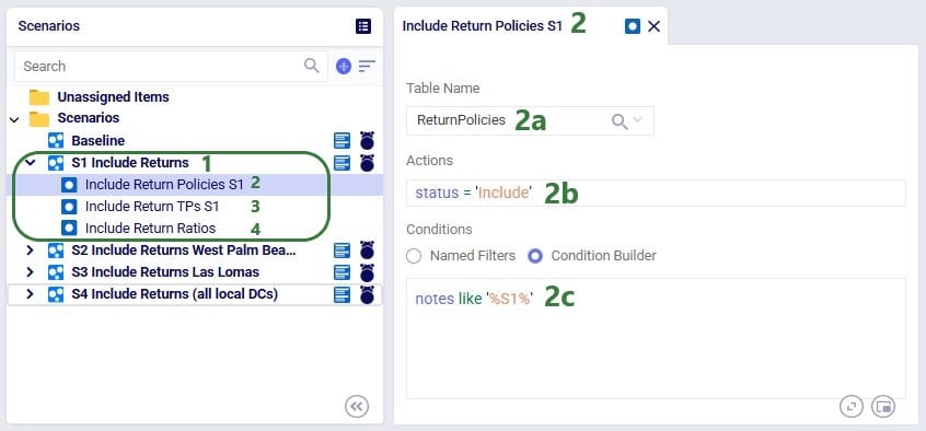
Now that we have populated the input tables to capture returns, we can set up scenario S1 which will change the Status of the appropriate records in these tables from Exclude to Include:
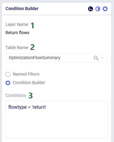
After running this scenario S1, we are first having a look at the map, where we will be showing the DCs, Customers and the Return Flows for scenario S1. This has been set up in the map named Supply Chain (S1) in the model from the Resource Library. To set this map up, we first copied the Supply Chain (Baseline) map and renamed it to Supply Chain (S1). Then clicked on the map’s name (Supply Chain (S1)) to open it and in the Map Filters form that is showing on the right-hand side of the screen changed the scenario to “S1 Include Returns” in the Scenario drop-down. To configure the Return Flows, we added a new Map Layer, and configured its Condition Builder form as follows (learn more about Maps and how to configure them in this Help Center article):
The resulting map is shown in this next screenshot:
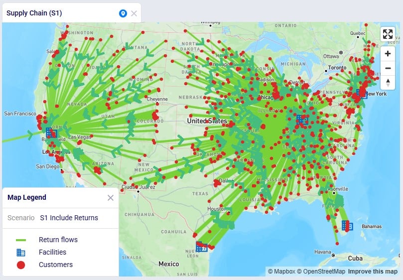
We see that, as expected, the bulk of the returns are going back the main DC in Cincinnati: from its local customers, but also from the customers served by the 2 smaller DCs in Las Lomas and West Palm Beach DCs. The customers served by the Clovis and Jersey City DCs return their products to their local DCs.
To assess the financial impact of including returns in the model, we again look at the Financials: Scenario Cost Comparison chart in the Optimization Scenario Comparison dashboard, comparing the S1 scenario to the Baseline scenario:

We see that including returns in S1 leads to:
Seeing that the main driver for the overall supply chain costs being higher when including returns are the high transportation costs for returning products, especially those travelling long distances from the Las Lomas and West Palm Beach customers to the Cincinnati DC sparks the idea to explore if it would be more beneficial for the Las Lomas and/or West Palm Beach customers to return their products to their local DC, rather than the Cincinnati DC. This will be modelled in the next three scenarios.
Building upon scenario S1, we will run 2 scenarios (S2 and S3) where it will be examined if it is beneficial cost-wise for West Palm Beach customers to return their products to their local West Palm Beach DC (S2) and for Las Lomas customers to return their products to their local Las Lomas DC (S3) rather than to the Cincinnati DC. In order to be able to handle returns, the fixed operating costs at these DCs are increased by 0.5M to 3.5M:

Scenarios S2 and S3 are run, and first we look at the map to check the return flows for the West Palm Beach and Las Lomas customers, respectively (copied the map for S1, renamed it, and then changed the scenario by clicking on the map’s name and selecting the S2/S3 scenario from the Scenario drop-down in the Map Filters pane on the right-hand side):
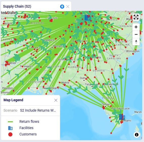
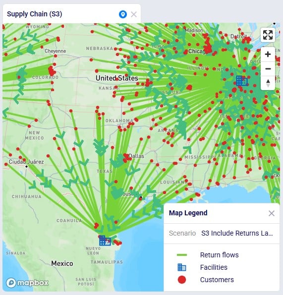
As expected, due to how we set up these scenarios, now all returns from these customers go to their local DC, rather than to DC-Cincinnati which was the case in scenario S1.
Let us next look at the overall costs for these 2 scenarios and compare them back to the S1 and Baseline scenarios:
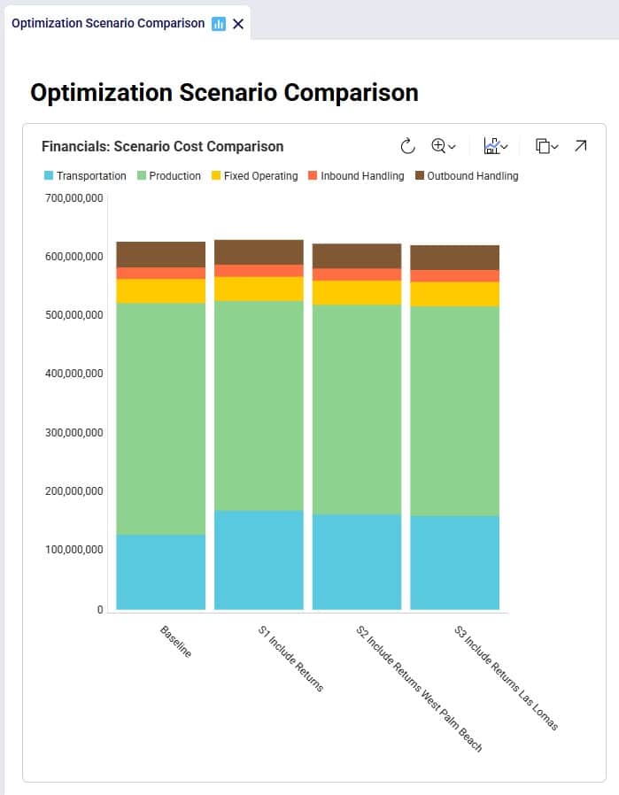
Besides some smaller reductions in the inbound and outbound costs in S2 and S3 as compared to S1, the transportation costs are reduced by sizeable amounts: 6.9M (S2 compared to S1) and 9.4M (S3 compared to S1), while the production (= procurement) costs are the same across these 3 scenarios. The reduction in transportation costs outweighs the 0.5M increase in fixed operating costs to be able to handle returns at the West Palm Beach and Las Lomas DCs. Also note that both scenario S2 and S3 have a lower total cost than the Baseline scenario.
Since it is beneficial to have the West Palm Beach and Las Lomas DCs handle returns, scenario S4 where this capability is included for both DCs is set up and run:
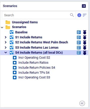
The S4 scenario increases the fixed operating costs at both these DCs from 3M to 3.5M (scenario items “Incr Operating Cost S2” and “Incr Operating Cost S3”), sets the Status of all records on the Return Ratios table to Include (the Include Return Ratios scenario item), and sets the Status to Include for records on the Return Policies and Transportation Policies tables where the Notes field contains the text “S4” (the “Include Return Policies S4” and “Include Return TPs S4” items), which are records where customers all ship their returns back to their local DC. We first check on the map if this is working as expected after running the S4 scenario:
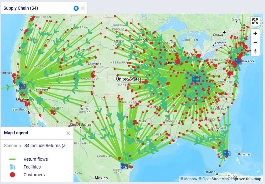
We notice that indeed there are no more returns going back to the Cincinnati DC from Las Lomas or West Palm Beach customers.
Finally, we expect the costs of this scenario to be the lowest overall since we should see the combined reductions of scenarios S2 and S3:
Between S1 and S4:
In addition to looking at maps or graphs, users can also use the output tables to understand the overall costs and flows, including those of the returns included in the network.
Often, users will start by looking at the overall cost picture using the Optimization Network Summary output table, which summarizes total costs and quantities at the scenario level:
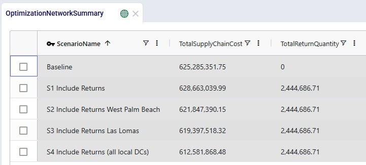
For each scenario, we are showing the Total Supply Chain Cost and Total Return Quantity fields here. As mentioned, the Baseline did not include any returns, whereas scenarios S1-4 did, which is reflected in the Total Return Quantity values. There are many more fields available on this output table, but in the next screenshot we are just showing the individual cost buckets that are used in this model (all other cost fields are 0):
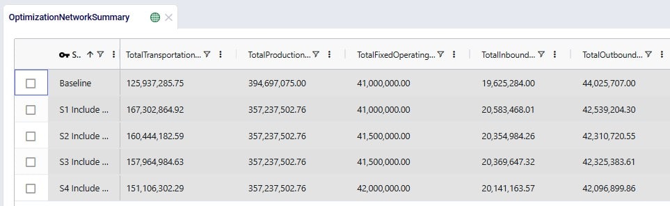
How these costs increase/decrease between scenarios has been discussed above when looking at the “Financials: Scenario Cost Comparison” chart in the “Optimization Scenario Comparison” dashboard. In summary:
Please note that on this table, there is also a Total Return Cost field. It is 0 in this example model. It would be > 0 if the Unit Cost field on the Return Policies table had been populated, which is a field where any specific cost related to the return can be captured. In our example Returns model, the return costs are entirely captured by the transportation costs and fixed operating costs specified.
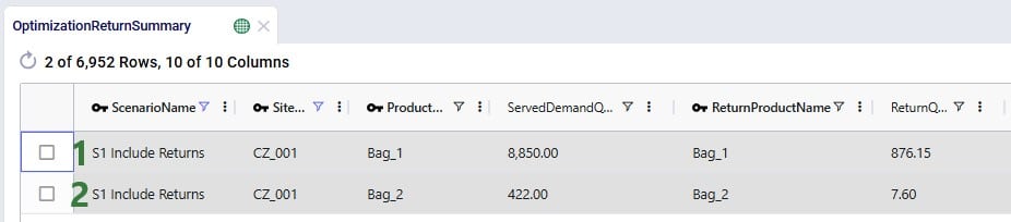
The Optimization Return Summary output table is a new output table that has been added to summarize returns at the scenario-returning site-product-return product-period level:
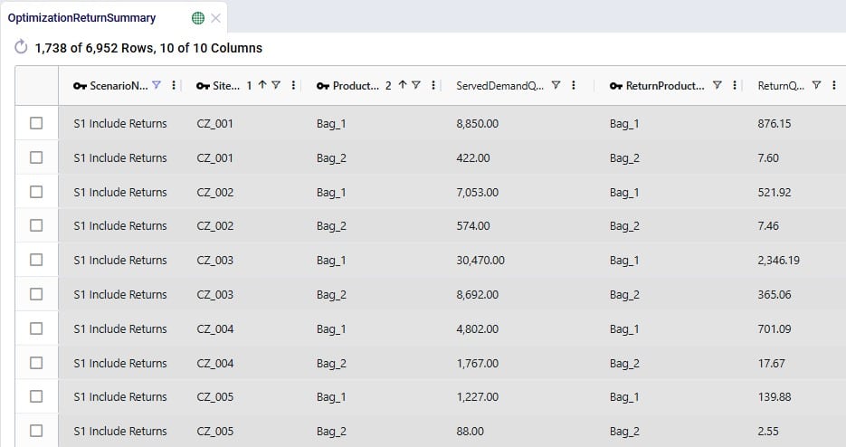
Looking at the first record here, we understand that in the S1 scenario, CZ_001 was served 8,850 units of Bag_1, while 876.15 units of Bag_1 were returned.
Lastly, we can also see individual return flows in the Optimization Flow Summary table by filtering the Flow Type field for “Return”:
Note that the product name for these flows is of the product that is being returned.
The example Returns model described above assumes that 100% of the returned Bag_1 and Bag_2 products can be reused. Here we will discuss through screenshots how the model can be adjusted to take into account that only 70% of Bag_1 returns and 50% of Bag_2 returns can be reused. To achieve this, we will need to add an additional “return” product for each finished good, set up bills of materials, and add records to the policies tables for the required additional model structure.
The tables that will be updated and for which we will see a screenshot each below are: Products, Groups, Return Policies, Return Ratios, Transportation Policies, Warehousing Policies, Bills of Materials, and Production Policies.
Two products are added here, 1 for each finished good: Bag_1_Return and Bag_2_Return. This way we can distinguish the return product from the sellable finished goods, apply different policies/costs to them, and convert a percentage back into the sellable items. The naming convention of adding “_Return” to the finished good name makes for easy filtering and provides clarity around what the product’s role is in the model. Of course, users can use different naming conventions.
The same unit value as for the finished goods is used for the return products, so that inventory carrying cost calculations are consistent. A unit price (again, same as the finished goods) has been entered too, but this will not actually be used by the model as these “_Return” products are not used to serve customer demand.

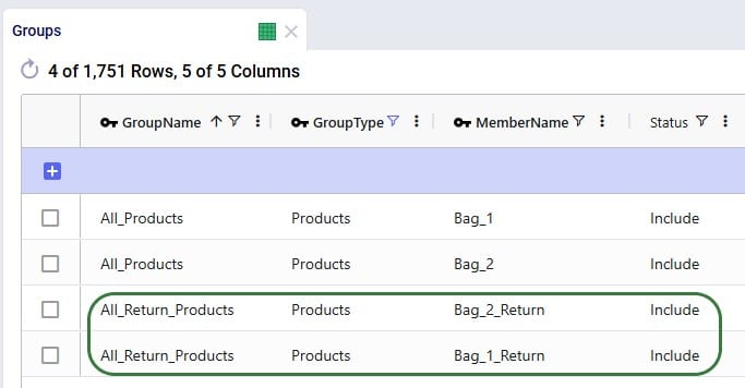
To facilitate setting up policies where the return products behave the same (e.g. same lanes, same costs, etc.), we add an “All_Return_Products” group to the Groups table, which consists of the 2 return products:
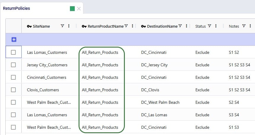
In the Return Policies table, the Return Product Name column needs to be updated to reflect that the products that are being returned are the “_Return” products. Previously, the Return Product Name was set to the All_Products group for each record, and it is now updated to the All_Return_Products group. Updating a field in all records or a subset of filtered records to the same value can be done using the Bulk Update Column functionality, which can be accessed by clicking on the icon with 3 vertical dots to the right of the column name and then choosing “Bulk Update this Column” in the list of options that comes up.
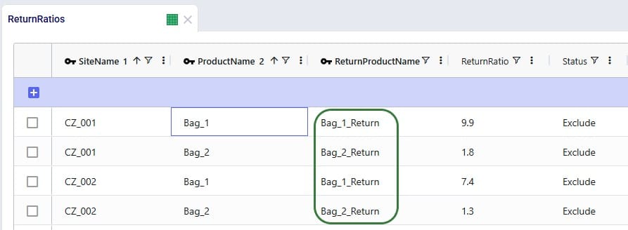
We keep the ratios of how much product comes back for each unit of Bag_1 / Bag_2 sold the same, however we need to update the Return Product Name field on all records to reflect that it is the “_Return” product that comes back. Since this table does not use groups because the return ratios are different for different customer-finished good combinations, the best way to update this table is to also use the bulk update column functionality:
Note that only 4 of the 1,738 records in this table are shown in the screenshot below.
Here, the records representing the lane back from the customers to the DC they send returns back to need to be updated so that the products going back are the “_Return” ones. Since the transportation costs of the return products are the same, we can keep using the grouped policies and just bulk update the Product Name column of the records where Mode Name equals Returns: change the values from the All_Products group to the All_Return_Products group.
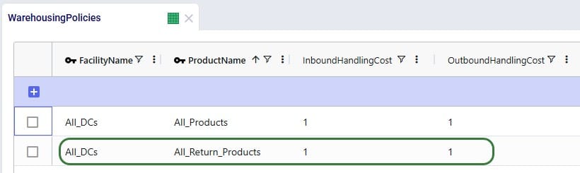
We want to apply the same inbound and outbound handling costs for the return products as we do for the finished goods, so a record is added for the “All_Return_Products” group at All_DCs in the Warehousing Policies table:
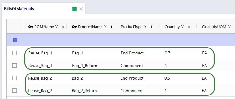
We can use the Bills of Materials (BOM) table to convert the “_Return” products back into the finished goods, applying the desired percentage that will be suitable for reuse. For Bag_1, we want to set up that 70% of the returns can be reused as finished goods, this is done by setting up a BOM as follows (the first 2 records in the screenshot below):
Similarly, we set up the BOM “Reuse_Bag_2” where 1 unit of Bag_2_Return results in 0.5 units of Bag_2 (the 3rd and 4th record in the screenshot):
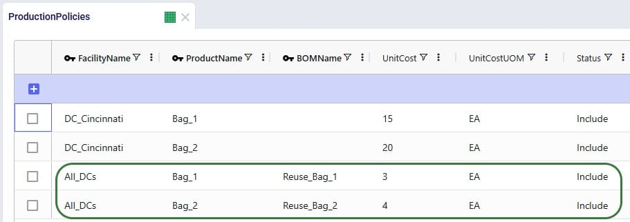
For the BOMs to be used, they need to be associated with the appropriate location-product combinations through production policies. So, we add 2 records to the Production Policies table, which set that at All_DCs the finished goods can be produced using the 2 BOMs. The Unit Cost set on this table represents the cost of inspecting each returned bag and deciding whether it can be reused.
With all the changes made on the input side, we can run the S1 Include Returns scenario (which was copied and renamed to “S1 Include Returns w BOM”). We will briefly look at how these changes affect the outputs.
In the Optimization Return Summary output table, users will notice that the Product Name is still either Bag_1 or Bag_2, but that the Return Product Name is either Bag_1_Return (for Bag_1) or Bag_2_Return (for Bag_2). The quantities are the same as before, since the return ratios are unchanged.

When looking at records of Flow Type = Return, we now see that the Product Name on these flows is that of the “_Return” products.

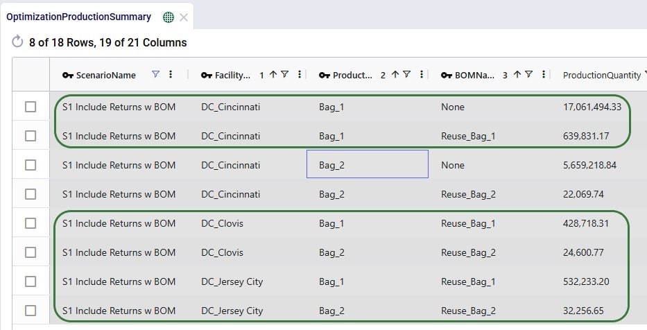
In this output table, we see that Bag_1 and Bag_2 are no longer only originating from the main DC in Cincinnati, but also at the 2 bigger local DCs that accept returns (Clovis, CA, and Jersey City, NJ) where a percentage of the returns is converted back into sellable finished goods through the BOMs.
In this appendix we will cover all fields on the 2 new input tables and the 1 new output table.

For various reasons, many supply chains need to deal with returns. This can for example be due to packaging materials coming back to be reused at plants or DCs, retail customers returning finished goods that they are not happy with, defective products, etc. Previously, these returns could mostly be modelled within Cosmic Frog NEO (Network Optimization) models by using some tricks and workarounds. But with the latest Cosmic Frog release, returns are now supported natively, so that the reuse, repurposing, or recycling of these retuned products to help companies reduce costs, minimize waste, and improve overall supply chain efficiency can be taken into account easily.
This documentation will first provide an overview of how returns work in a Cosmic Frog model and then walk through an example model of a retailer which includes modelling the returns of finished goods. The appendix details all the new returns-related fields in several new tables and some of the existing tables.
When modelling returns in Cosmic Frog:
Users need to use 2 new input tables to set up returns:
The Return Ratios table contains the information on how much return-product is returned for a certain amount of product delivered to a certain destination:
The Return Policies table is used to indicate where returned products need to go to and the rules around multiple possible destinations. Optionally, costs can be associated with the returns here and a maximum distance allowed for returns can be entered on this table too.
Note that both these tables have Status and Notes fields (not shown in the screenshots), like most Cosmic Frog input tables have. These are often used for scenario creation where the Status is set to Exclude in the table itself and changed to Include in select scenarios based on text in the Notes field.
All columns on these 2 returns-related input table are explained in more detail in the appendix.
In addition to populating the Return Policies and Return Ratios tables, users need to be aware that additional model structure needed for the returned products may need to be put in place:
The Optimization Return Summary output table is a new output table that will be generated for Neo runs if returns are included in the modelling:
This table and all its fields are explained in detail in the appendix.
The Optimization Flow Summary output table will contain additional records for models that include returns; they can be identified by filtering the Flow Type field for “Return”:
These 2 records show the return flows and associated transportation costs for the Bag_1 and Bag_2 products from CZ_001, going to DC_Cincinnati, that we saw in the Optimization Return Summary table screenshot above.
In addition to the new Optimization Return Summary output table, and new records of Flow Type = Return in the Optimization Flow Summary output table, following existing output tables now contain additional fields related to returns:
The example Returns model can be copied from the Resource Library to a user’s Optilogic account (see this help center article on how to use the Resource Library). It models the US supply chain of a fashion bag retailer. The model’s locations and flows both to customers and between DCs are shown in this screenshot (returns are not yet included here):
Historically, the retailer had 1 main DC in Cincinnati, Ohio, where all products were received and all 869 customers were fulfilled from. Over time, 4 secondary DCs were added based on Greenfield analysis, 2 bigger ones in Clovis, California, and Jersey City, New Jersey, and 2 smaller ones in West Palm Beach, Florida, and Las Lomas, Texas. These secondary DCs receive product from the Cincinnati DC and serve their own set of customers. The main DC in Cincinnati and the 2 bigger secondary DCs (Clovis, CA, and Jersey City, NJ) can handle returns currently: returns are received there and re-used to fulfill demand. However, until now, these returns had not been taken into account in the modelling. In this model we will explore following scenarios:
Other model features:
Please note that in this model the order of columns in the tables has sometimes been changed to put those containing data together on the left-hand side of the table. All columns are still present in the table but may be in a different position than you are used to. Columns can be reset to their default position by choosing “Reset Columns” from the menu that comes up when clicking on the icon with 3 vertical dots to the right of a column name.
After running the baseline scenario (which does not include returns), we take a look at the Financials: Scenario Cost Comparison chart in the Optimization Scenario Comparison dashboard (in Cosmic Frog’s Analytics module):
We see that the biggest cost currently is the production cost at 394.7M (= procurement of all product into Cincinnati), followed by transportation costs at 125.9M. The total supply chain cost of this scenario is 625.3M.
In this scenario we want to include how returns currently work: Cincinnati, Clovis, and Jersey City customers return their products to their local DCs whereas West Palm Beach and Las Lomas customers return their products to the main DC in Cincinnati. To set this up, we need to add records to the Return Policies, Return Ratios, and Transportation Policies input tables. To not change the Baseline scenario, all new records will be added with Status = Exclude, and the Notes field populated so it can be used to filter on in scenario items that change the Status to Include for subsets of records. Starting with the Return Policies table:
Next, we need to add records to the Transportation Policies table so that there is at least 1 lane available for each site-product-destination combination set up in the return policies table. For this example, we add records to the Transportation Policies table that match the ones added to the Return Policies table exactly, while additionally setting Mode Name = Returns, Unit Cost = 0.04 and Unit Cost UOM = EA-MI (the latter is not shown in the screenshot below), which means the transportation cost on return lanes is 0.04 per unit per mile:
Finally, we also need to indicate how much product is returned in the Return Ratios table. Since we want to model different ratios by individual customer and individual product, this table does not use any groups. Groups can however be used in this table too for the Site Name, Product Name, Period Name, and Return Product Name fields.
Please note that adding records to these 3 tables and including them in the scenarios is sufficient to capture returns in this example model. For other models it is possible that additional tables may need to be used, see the Other Input Tables section above.
Now that we have populated the input tables to capture returns, we can set up scenario S1 which will change the Status of the appropriate records in these tables from Exclude to Include:
After running this scenario S1, we are first having a look at the map, where we will be showing the DCs, Customers and the Return Flows for scenario S1. This has been set up in the map named Supply Chain (S1) in the model from the Resource Library. To set this map up, we first copied the Supply Chain (Baseline) map and renamed it to Supply Chain (S1). Then clicked on the map’s name (Supply Chain (S1)) to open it and in the Map Filters form that is showing on the right-hand side of the screen changed the scenario to “S1 Include Returns” in the Scenario drop-down. To configure the Return Flows, we added a new Map Layer, and configured its Condition Builder form as follows (learn more about Maps and how to configure them in this Help Center article):
The resulting map is shown in this next screenshot:
We see that, as expected, the bulk of the returns are going back the main DC in Cincinnati: from its local customers, but also from the customers served by the 2 smaller DCs in Las Lomas and West Palm Beach DCs. The customers served by the Clovis and Jersey City DCs return their products to their local DCs.
To assess the financial impact of including returns in the model, we again look at the Financials: Scenario Cost Comparison chart in the Optimization Scenario Comparison dashboard, comparing the S1 scenario to the Baseline scenario:
We see that including returns in S1 leads to:
Seeing that the main driver for the overall supply chain costs being higher when including returns are the high transportation costs for returning products, especially those travelling long distances from the Las Lomas and West Palm Beach customers to the Cincinnati DC sparks the idea to explore if it would be more beneficial for the Las Lomas and/or West Palm Beach customers to return their products to their local DC, rather than the Cincinnati DC. This will be modelled in the next three scenarios.
Building upon scenario S1, we will run 2 scenarios (S2 and S3) where it will be examined if it is beneficial cost-wise for West Palm Beach customers to return their products to their local West Palm Beach DC (S2) and for Las Lomas customers to return their products to their local Las Lomas DC (S3) rather than to the Cincinnati DC. In order to be able to handle returns, the fixed operating costs at these DCs are increased by 0.5M to 3.5M:
Scenarios S2 and S3 are run, and first we look at the map to check the return flows for the West Palm Beach and Las Lomas customers, respectively (copied the map for S1, renamed it, and then changed the scenario by clicking on the map’s name and selecting the S2/S3 scenario from the Scenario drop-down in the Map Filters pane on the right-hand side):
As expected, due to how we set up these scenarios, now all returns from these customers go to their local DC, rather than to DC-Cincinnati which was the case in scenario S1.
Let us next look at the overall costs for these 2 scenarios and compare them back to the S1 and Baseline scenarios:
Besides some smaller reductions in the inbound and outbound costs in S2 and S3 as compared to S1, the transportation costs are reduced by sizeable amounts: 6.9M (S2 compared to S1) and 9.4M (S3 compared to S1), while the production (= procurement) costs are the same across these 3 scenarios. The reduction in transportation costs outweighs the 0.5M increase in fixed operating costs to be able to handle returns at the West Palm Beach and Las Lomas DCs. Also note that both scenario S2 and S3 have a lower total cost than the Baseline scenario.
Since it is beneficial to have the West Palm Beach and Las Lomas DCs handle returns, scenario S4 where this capability is included for both DCs is set up and run:
The S4 scenario increases the fixed operating costs at both these DCs from 3M to 3.5M (scenario items “Incr Operating Cost S2” and “Incr Operating Cost S3”), sets the Status of all records on the Return Ratios table to Include (the Include Return Ratios scenario item), and sets the Status to Include for records on the Return Policies and Transportation Policies tables where the Notes field contains the text “S4” (the “Include Return Policies S4” and “Include Return TPs S4” items), which are records where customers all ship their returns back to their local DC. We first check on the map if this is working as expected after running the S4 scenario:
We notice that indeed there are no more returns going back to the Cincinnati DC from Las Lomas or West Palm Beach customers.
Finally, we expect the costs of this scenario to be the lowest overall since we should see the combined reductions of scenarios S2 and S3:
Between S1 and S4:
In addition to looking at maps or graphs, users can also use the output tables to understand the overall costs and flows, including those of the returns included in the network.
Often, users will start by looking at the overall cost picture using the Optimization Network Summary output table, which summarizes total costs and quantities at the scenario level:
For each scenario, we are showing the Total Supply Chain Cost and Total Return Quantity fields here. As mentioned, the Baseline did not include any returns, whereas scenarios S1-4 did, which is reflected in the Total Return Quantity values. There are many more fields available on this output table, but in the next screenshot we are just showing the individual cost buckets that are used in this model (all other cost fields are 0):
How these costs increase/decrease between scenarios has been discussed above when looking at the “Financials: Scenario Cost Comparison” chart in the “Optimization Scenario Comparison” dashboard. In summary:
Please note that on this table, there is also a Total Return Cost field. It is 0 in this example model. It would be > 0 if the Unit Cost field on the Return Policies table had been populated, which is a field where any specific cost related to the return can be captured. In our example Returns model, the return costs are entirely captured by the transportation costs and fixed operating costs specified.
The Optimization Return Summary output table is a new output table that has been added to summarize returns at the scenario-returning site-product-return product-period level:
Looking at the first record here, we understand that in the S1 scenario, CZ_001 was served 8,850 units of Bag_1, while 876.15 units of Bag_1 were returned.
Lastly, we can also see individual return flows in the Optimization Flow Summary table by filtering the Flow Type field for “Return”:
Note that the product name for these flows is of the product that is being returned.
The example Returns model described above assumes that 100% of the returned Bag_1 and Bag_2 products can be reused. Here we will discuss through screenshots how the model can be adjusted to take into account that only 70% of Bag_1 returns and 50% of Bag_2 returns can be reused. To achieve this, we will need to add an additional “return” product for each finished good, set up bills of materials, and add records to the policies tables for the required additional model structure.
The tables that will be updated and for which we will see a screenshot each below are: Products, Groups, Return Policies, Return Ratios, Transportation Policies, Warehousing Policies, Bills of Materials, and Production Policies.
Two products are added here, 1 for each finished good: Bag_1_Return and Bag_2_Return. This way we can distinguish the return product from the sellable finished goods, apply different policies/costs to them, and convert a percentage back into the sellable items. The naming convention of adding “_Return” to the finished good name makes for easy filtering and provides clarity around what the product’s role is in the model. Of course, users can use different naming conventions.
The same unit value as for the finished goods is used for the return products, so that inventory carrying cost calculations are consistent. A unit price (again, same as the finished goods) has been entered too, but this will not actually be used by the model as these “_Return” products are not used to serve customer demand.
To facilitate setting up policies where the return products behave the same (e.g. same lanes, same costs, etc.), we add an “All_Return_Products” group to the Groups table, which consists of the 2 return products:
In the Return Policies table, the Return Product Name column needs to be updated to reflect that the products that are being returned are the “_Return” products. Previously, the Return Product Name was set to the All_Products group for each record, and it is now updated to the All_Return_Products group. Updating a field in all records or a subset of filtered records to the same value can be done using the Bulk Update Column functionality, which can be accessed by clicking on the icon with 3 vertical dots to the right of the column name and then choosing “Bulk Update this Column” in the list of options that comes up.
We keep the ratios of how much product comes back for each unit of Bag_1 / Bag_2 sold the same, however we need to update the Return Product Name field on all records to reflect that it is the “_Return” product that comes back. Since this table does not use groups because the return ratios are different for different customer-finished good combinations, the best way to update this table is to also use the bulk update column functionality:
Note that only 4 of the 1,738 records in this table are shown in the screenshot below.
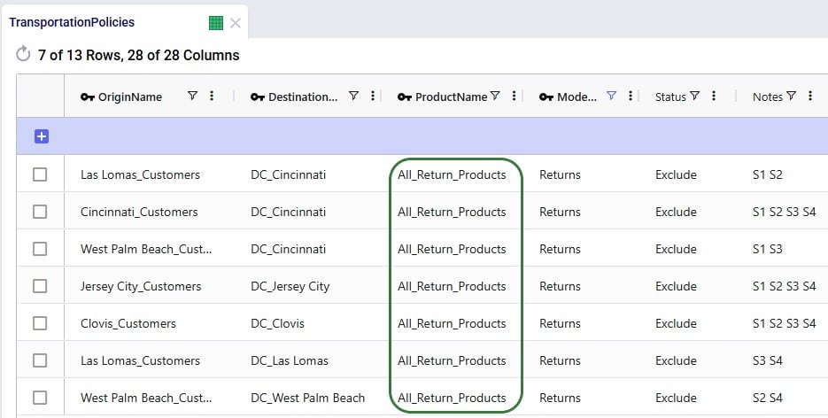
Here, the records representing the lane back from the customers to the DC they send returns back to need to be updated so that the products going back are the “_Return” ones. Since the transportation costs of the return products are the same, we can keep using the grouped policies and just bulk update the Product Name column of the records where Mode Name equals Returns: change the values from the All_Products group to the All_Return_Products group.
We want to apply the same inbound and outbound handling costs for the return products as we do for the finished goods, so a record is added for the “All_Return_Products” group at All_DCs in the Warehousing Policies table:
We can use the Bills of Materials (BOM) table to convert the “_Return” products back into the finished goods, applying the desired percentage that will be suitable for reuse. For Bag_1, we want to set up that 70% of the returns can be reused as finished goods, this is done by setting up a BOM as follows (the first 2 records in the screenshot below):
Similarly, we set up the BOM “Reuse_Bag_2” where 1 unit of Bag_2_Return results in 0.5 units of Bag_2 (the 3rd and 4th record in the screenshot):
For the BOMs to be used, they need to be associated with the appropriate location-product combinations through production policies. So, we add 2 records to the Production Policies table, which set that at All_DCs the finished goods can be produced using the 2 BOMs. The Unit Cost set on this table represents the cost of inspecting each returned bag and deciding whether it can be reused.
With all the changes made on the input side, we can run the S1 Include Returns scenario (which was copied and renamed to “S1 Include Returns w BOM”). We will briefly look at how these changes affect the outputs.
In the Optimization Return Summary output table, users will notice that the Product Name is still either Bag_1 or Bag_2, but that the Return Product Name is either Bag_1_Return (for Bag_1) or Bag_2_Return (for Bag_2). The quantities are the same as before, since the return ratios are unchanged.
When looking at records of Flow Type = Return, we now see that the Product Name on these flows is that of the “_Return” products.
In this output table, we see that Bag_1 and Bag_2 are no longer only originating from the main DC in Cincinnati, but also at the 2 bigger local DCs that accept returns (Clovis, CA, and Jersey City, NJ) where a percentage of the returns is converted back into sellable finished goods through the BOMs.
In this appendix we will cover all fields on the 2 new input tables and the 1 new output table.