Being able to assess the Risk associated with your supply chain has increasingly become more important in a quickly changing world with high levels of volatility. Not only does Cosmic Frog calculate an overall supply chain risk score for each scenario that is run, but it also gives you details about the risk at the location and flow level, so you can easily identify the highest and lowest risk components of your supply chain and use that knowledge to quickly set up new scenarios to reduce the risk in your network.
By default, any Neo optimization, Triad greenfield or Throg simulation model run will have the default risk settings, called OptiRisk, applied using the DART risk engine. See also the Getting Started with the Optilogic Risk Engine documentation. Here we will cover how a Cosmic Frog user can set up their own risk profile(s) to rate the risk of the locations and flows in the network and that of the overall network. Inputs and outputs are covered and in the last section notes & tips & additional resources are listed.
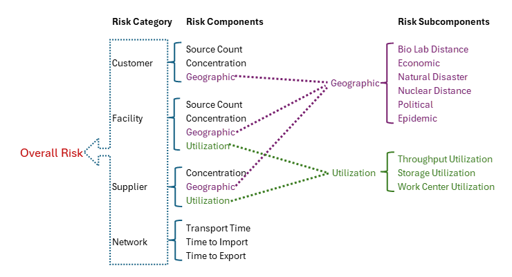
The following diagram shows the Cosmic Frog risk categories, their components, and subcomponents.
A description of these risk components and subcomponents follows here:
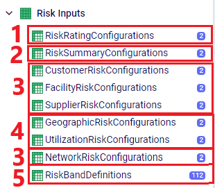
Custom risk profiles are set up and configured using the following 9 tables in the Risk Inputs section of Cosmic Frog’s input tables. These 9 input tables can be divided into 5 categories:
Following is a summary of these table categories; more details on individual tables will be discussed below:
We will cover some of the individual Risk Input tables in more detail now, starting with the Risk Rating Configurations table:

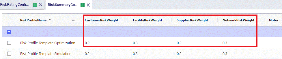
In the Risk Summary Configurations table, we can set the weights for the 4 different risk components that will be used to calculate the overall Risk Score of the supply chain. The 4 components are: customers, facilities, suppliers, and network. In the screenshot below, customer and supplier risk are contributing 20% each to the overall risk score while facility and network risk are contributing 30% each to the overall risk score.
These 4 weights should add up to 1 (=100%). If they do not add up to 1, Cosmic Frog will still run and automatically scale the Risk Score up or down as needed. For example, if the weights add up to 0.9, the final Risk Score that is calculated based on these 4 risk categories and their weights will be divided by 0.9 to scale it up to 100%. In other words, the weight of each risk category is multiplied by 1/0.9 = 1.11 so that the weights then add up to 100% instead of 90%. If you do not want to use a certain risk category in the Risk Score calculation, you can set its weight to 0. Note that you cannot leave a weight field blank. These rules around automatically scaling weights up or down to add up to 1 and setting a weight to 0 if you do not want to use that specific risk component or subcomponent also apply to the other “… Risk Configurations” tables.
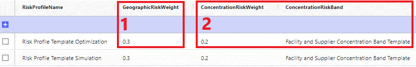
Following are 2 screenshots of the Facility Risk Configurations table on which the weights and risk bands to calculate the Risk Score for individual facility locations are specified. A subset of these same risk components is also used for customers (Customer Risk Configurations table) and suppliers (Supplier Risk Configurations table). We will not discuss those 2 tables in detail in this documentation since they work in the same way as described here for facilities.
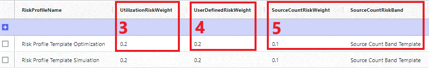
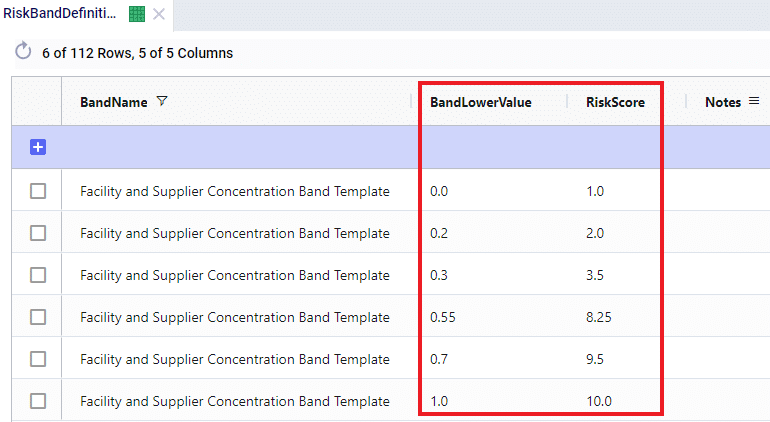
The first band is from 0.0 (first Band Lower Value) to 0.2 (the next Band Lower Value), meaning between 0% and 20% of total network throughput at an individual facility. The risk score for 0% of total network throughput is 1.0 and goes up to 2.0 when total network throughput at the facility goes up to 20%. For facilities with a concentration (= % of total network throughput) between 0 and 20%, the Risk Score will be linearly interpolated from the lower risk score of 1.0 to the higher risk score of 2.0. For example, a facility that has 5% of total network throughput will have a concentration risk score of 1.25. The next band is for 20%-30% of total network throughput, with an associated risk between 2.0 and 3.5, etc. Finally, if all network throughput is at only 1 location (Band Lower Value = 1.0), the risk score for that facility is 10.0. The risk scores for any band run from 1, lowest risk, to 10, highest risk.
Following screenshot shows the Geographic Risk Configurations table with 2 of its risk subcomponents, biolab distance and economic:
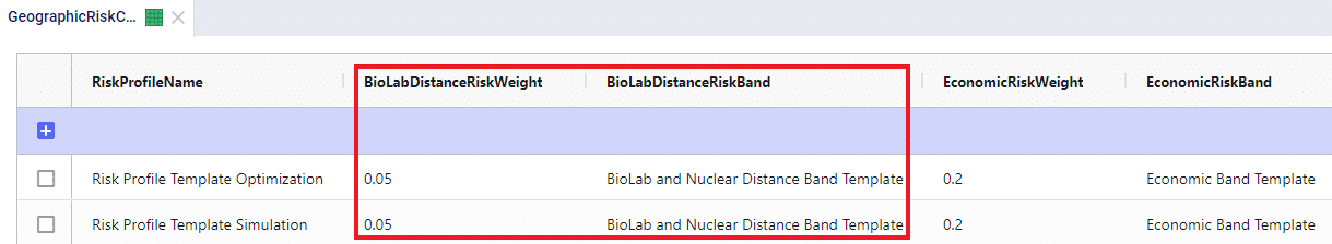
As an example here in the red outline, the Biolab Distance Risk is specified by setting its weight to 0.05 or 5% and specifying which band definition on the Risk Band Definitions table should be used, which is “BioLab and Nuclear Distance Band Template”. The Definition of this band template is as follows when looked up in the Risk Band Definitions table:
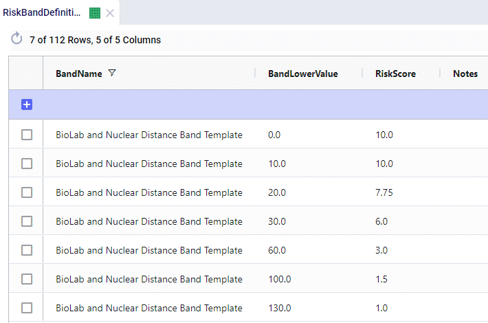
This band definition says that if a location is within 0-10 miles to a Biolab of Safety Level 4, the Risk Score is 10.0. A distance of 10-20 miles has an associated Risk Score between 10 and 7.75, etc. If a location is 130 miles or farther from a biolab of safety Level 4, the Risk Score is 1.0.
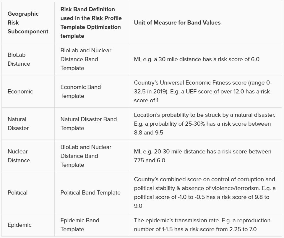
The other 5 subcomponents of Geographic Risk are defined in a similar manner on this table: with a Risk Weight field and a Risk Band field that specifies which Band Definition on the Risk Band Definitions table is to be used for that risk subcomponent. The following table summarizes the names of the Band Definitions used for these geographic risk subcomponents and what the unit of measure is for the Band Values with an example:
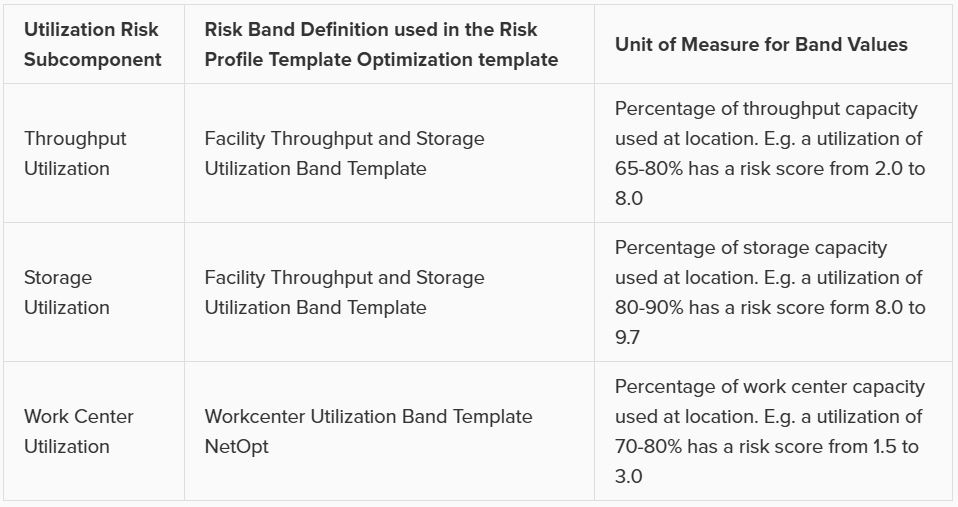
Similar to the Geographic Risk component, the Utilization Risk component also has its own table, Utilization Risk Configurations, where its 3 risk subcomponents are configured. Again, each of the subcomponents has a Risk Weight field and a Risk Band field associated with it. The following table summarizes the names of the Band Definitions used for these utilization risk subcomponents and what the unit of measure is for the Band Values with an example:
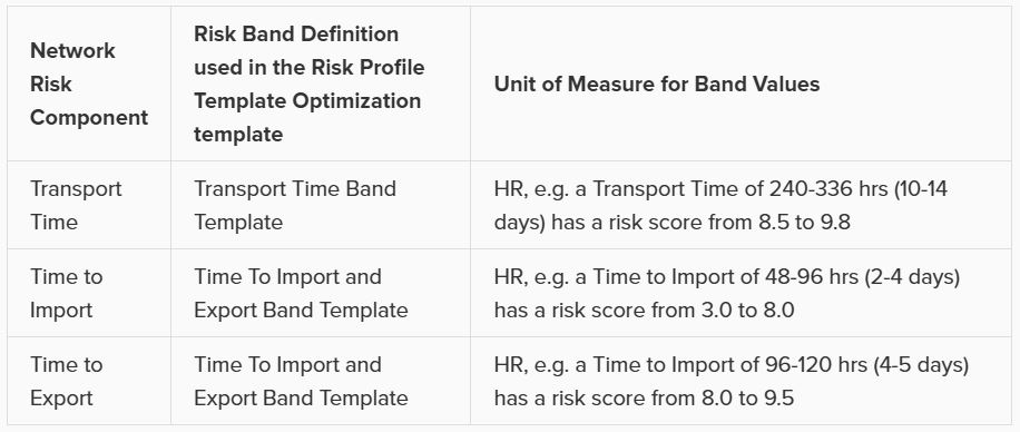
Lastly on the Risk Inputs side, the Network Risk Configurations table specifies the components of Network Risk in a similar manner: with a Risk Weight and a Risk Band field for each risk component. The following table summarizes the names of the Band Definitions used for these network risk subcomponents and what the unit of measure is for the Band Values with an example:
Risk outputs can be found in some of the standard Output Summary Tables and in the risk specific Output Risk Tables:

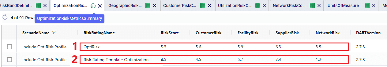
The following screenshot shows the Optimization Risk Metrics Summary output table for a scenario called “Include Opt Risk Profile”. It shows both the OptiRisk and Risk Rating Template Optimization risk score outputs:
On the Optimization Customer Risk Metrics, Optimization Facility Risk Metrics, and Optimization Supplier Risk Metrics tables, the overall risk score for each customer, facility, and supplier can be found, respectively. They also show the risk scores of each risk component, e.g. for customers these components are Concentration Risk, Source Count Risk, and Geographic risk. The subcomponents for Geographic risk are further detailed in the Optimization Geographic Risk Metrics output table, where for each customer, facility, and supplier the overall geographic risk score and the risk scores of each of the geographic risk subcomponents are listed. Similarly, on the Facility Risk Metrics and Supplier Risk Metrics tables, the Utilization Risk score will be listed for each location, whilst the Optimization Utilization Risk Metrics table will detail the risk scores of the subcomponents of this risk (throughput utilization, storage utilization, and work center utilization).
Let’s walk through an example of how the risk score for the facility Plant_France_Paris_9904000 was calculated using a few screenshots of input and output tables. This first screenshot shows the Optimization Geographic Risk Metrics output table for this facility:

The geographic risk score of this facility is calculated as 4.0 and the values for all the geographic risk subcomponents are listed here too, for example 8.2 for biolab distance risk and 3.6 for political risk. The overall geographic risk of 4.0 was calculated using the risk score of each geographic risk subcomponent and the weights that are set on the Geographic Risk Configurations input table:
Geographic Risk Score = (biolab distance risk * biolab distance risk weight + economic risk * economic risk weight + natural disaster risk * natural disaster risk weight + nuclear distance risk * nuclear distance risk weight + political risk * political risk weight + epidemic risk * epidemic risk weight) / 0.8 = (8.2 * 0.05 + 5.3 * 0.2 + 2.8 * 0.3 + 2.3 * 0.05 + 3.6 * 0.1 + 4.5 * 0.1) / 0.8 = 4.0. (We need to divide by 0.8 since the weights do not add up to 1, but only to 0.8).
Next, in the Optimization Facility Risk Metrics output table we can see that the overall facility risk score is calculated as 6.8, which is the result of combining the concentration risk score, source count risk score, and geographic risk score using the weights set on the Facility Risk Configurations input table.
This screenshot shows the Facility Risk Configurations input table and the weights for the different risk components:
Facility Risk Score = (geographic risk * geographic risk weight + concentration risk * concentration risk weight + source count risk * source count risk weight) / 0.6 = 4.0 * 0.3 + 9.3 * 0.2 + 10.0 * 0.1) / 0.6 = 6.8. (We need to divide by 0.6 since the weights do not add up to 1, but only to 0.6).
A few things about Risk in Cosmic Frog that are good to keep in mind:

Being able to assess the Risk associated with your supply chain has increasingly become more important in a quickly changing world with high levels of volatility. Not only does Cosmic Frog calculate an overall supply chain risk score for each scenario that is run, but it also gives you details about the risk at the location and flow level, so you can easily identify the highest and lowest risk components of your supply chain and use that knowledge to quickly set up new scenarios to reduce the risk in your network.
By default, any Neo optimization, Triad greenfield or Throg simulation model run will have the default risk settings, called OptiRisk, applied using the DART risk engine. See also the Getting Started with the Optilogic Risk Engine documentation. Here we will cover how a Cosmic Frog user can set up their own risk profile(s) to rate the risk of the locations and flows in the network and that of the overall network. Inputs and outputs are covered and in the last section notes & tips & additional resources are listed.
The following diagram shows the Cosmic Frog risk categories, their components, and subcomponents.
A description of these risk components and subcomponents follows here:
Custom risk profiles are set up and configured using the following 9 tables in the Risk Inputs section of Cosmic Frog’s input tables. These 9 input tables can be divided into 5 categories:
Following is a summary of these table categories; more details on individual tables will be discussed below:
We will cover some of the individual Risk Input tables in more detail now, starting with the Risk Rating Configurations table:
In the Risk Summary Configurations table, we can set the weights for the 4 different risk components that will be used to calculate the overall Risk Score of the supply chain. The 4 components are: customers, facilities, suppliers, and network. In the screenshot below, customer and supplier risk are contributing 20% each to the overall risk score while facility and network risk are contributing 30% each to the overall risk score.
These 4 weights should add up to 1 (=100%). If they do not add up to 1, Cosmic Frog will still run and automatically scale the Risk Score up or down as needed. For example, if the weights add up to 0.9, the final Risk Score that is calculated based on these 4 risk categories and their weights will be divided by 0.9 to scale it up to 100%. In other words, the weight of each risk category is multiplied by 1/0.9 = 1.11 so that the weights then add up to 100% instead of 90%. If you do not want to use a certain risk category in the Risk Score calculation, you can set its weight to 0. Note that you cannot leave a weight field blank. These rules around automatically scaling weights up or down to add up to 1 and setting a weight to 0 if you do not want to use that specific risk component or subcomponent also apply to the other “… Risk Configurations” tables.
Following are 2 screenshots of the Facility Risk Configurations table on which the weights and risk bands to calculate the Risk Score for individual facility locations are specified. A subset of these same risk components is also used for customers (Customer Risk Configurations table) and suppliers (Supplier Risk Configurations table). We will not discuss those 2 tables in detail in this documentation since they work in the same way as described here for facilities.
The first band is from 0.0 (first Band Lower Value) to 0.2 (the next Band Lower Value), meaning between 0% and 20% of total network throughput at an individual facility. The risk score for 0% of total network throughput is 1.0 and goes up to 2.0 when total network throughput at the facility goes up to 20%. For facilities with a concentration (= % of total network throughput) between 0 and 20%, the Risk Score will be linearly interpolated from the lower risk score of 1.0 to the higher risk score of 2.0. For example, a facility that has 5% of total network throughput will have a concentration risk score of 1.25. The next band is for 20%-30% of total network throughput, with an associated risk between 2.0 and 3.5, etc. Finally, if all network throughput is at only 1 location (Band Lower Value = 1.0), the risk score for that facility is 10.0. The risk scores for any band run from 1, lowest risk, to 10, highest risk.
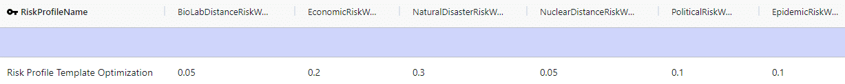
Following screenshot shows the Geographic Risk Configurations table with 2 of its risk subcomponents, biolab distance and economic:
As an example here in the red outline, the Biolab Distance Risk is specified by setting its weight to 0.05 or 5% and specifying which band definition on the Risk Band Definitions table should be used, which is “BioLab and Nuclear Distance Band Template”. The Definition of this band template is as follows when looked up in the Risk Band Definitions table:
This band definition says that if a location is within 0-10 miles to a Biolab of Safety Level 4, the Risk Score is 10.0. A distance of 10-20 miles has an associated Risk Score between 10 and 7.75, etc. If a location is 130 miles or farther from a biolab of safety Level 4, the Risk Score is 1.0.
The other 5 subcomponents of Geographic Risk are defined in a similar manner on this table: with a Risk Weight field and a Risk Band field that specifies which Band Definition on the Risk Band Definitions table is to be used for that risk subcomponent. The following table summarizes the names of the Band Definitions used for these geographic risk subcomponents and what the unit of measure is for the Band Values with an example:
Similar to the Geographic Risk component, the Utilization Risk component also has its own table, Utilization Risk Configurations, where its 3 risk subcomponents are configured. Again, each of the subcomponents has a Risk Weight field and a Risk Band field associated with it. The following table summarizes the names of the Band Definitions used for these utilization risk subcomponents and what the unit of measure is for the Band Values with an example:
Lastly on the Risk Inputs side, the Network Risk Configurations table specifies the components of Network Risk in a similar manner: with a Risk Weight and a Risk Band field for each risk component. The following table summarizes the names of the Band Definitions used for these network risk subcomponents and what the unit of measure is for the Band Values with an example:
Risk outputs can be found in some of the standard Output Summary Tables and in the risk specific Output Risk Tables:
The following screenshot shows the Optimization Risk Metrics Summary output table for a scenario called “Include Opt Risk Profile”. It shows both the OptiRisk and Risk Rating Template Optimization risk score outputs:
On the Optimization Customer Risk Metrics, Optimization Facility Risk Metrics, and Optimization Supplier Risk Metrics tables, the overall risk score for each customer, facility, and supplier can be found, respectively. They also show the risk scores of each risk component, e.g. for customers these components are Concentration Risk, Source Count Risk, and Geographic risk. The subcomponents for Geographic risk are further detailed in the Optimization Geographic Risk Metrics output table, where for each customer, facility, and supplier the overall geographic risk score and the risk scores of each of the geographic risk subcomponents are listed. Similarly, on the Facility Risk Metrics and Supplier Risk Metrics tables, the Utilization Risk score will be listed for each location, whilst the Optimization Utilization Risk Metrics table will detail the risk scores of the subcomponents of this risk (throughput utilization, storage utilization, and work center utilization).
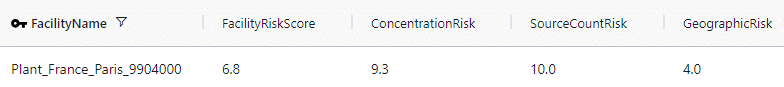
Let’s walk through an example of how the risk score for the facility Plant_France_Paris_9904000 was calculated using a few screenshots of input and output tables. This first screenshot shows the Optimization Geographic Risk Metrics output table for this facility:
The geographic risk score of this facility is calculated as 4.0 and the values for all the geographic risk subcomponents are listed here too, for example 8.2 for biolab distance risk and 3.6 for political risk. The overall geographic risk of 4.0 was calculated using the risk score of each geographic risk subcomponent and the weights that are set on the Geographic Risk Configurations input table:
Geographic Risk Score = (biolab distance risk * biolab distance risk weight + economic risk * economic risk weight + natural disaster risk * natural disaster risk weight + nuclear distance risk * nuclear distance risk weight + political risk * political risk weight + epidemic risk * epidemic risk weight) / 0.8 = (8.2 * 0.05 + 5.3 * 0.2 + 2.8 * 0.3 + 2.3 * 0.05 + 3.6 * 0.1 + 4.5 * 0.1) / 0.8 = 4.0. (We need to divide by 0.8 since the weights do not add up to 1, but only to 0.8).
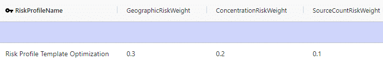
Next, in the Optimization Facility Risk Metrics output table we can see that the overall facility risk score is calculated as 6.8, which is the result of combining the concentration risk score, source count risk score, and geographic risk score using the weights set on the Facility Risk Configurations input table.
This screenshot shows the Facility Risk Configurations input table and the weights for the different risk components:
Facility Risk Score = (geographic risk * geographic risk weight + concentration risk * concentration risk weight + source count risk * source count risk weight) / 0.6 = 4.0 * 0.3 + 9.3 * 0.2 + 10.0 * 0.1) / 0.6 = 6.8. (We need to divide by 0.6 since the weights do not add up to 1, but only to 0.6).
A few things about Risk in Cosmic Frog that are good to keep in mind: